Download
1 / 25
270 likes | 491 Views
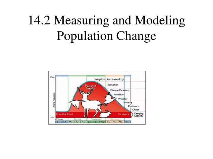
14.2 Measuring and Modeling Population Change. Carrying capacity. The maximum number of organisms that can be sustained by available resources over a given period of time Is dynamic because environmental conditions are always changing. Population growth: factors.

E N D
Carrying capacity • The maximum number of organisms that can be sustained by available resources over a given period of time • Is dynamic because environmental conditions are always changing
Population growth: factors Population dynamics: changes in population characteristics The main determinants are: • natality (birth rate) • mortality (death rate) • Immigration (individuals moving in) • Emigration (individuals moving out)
Population change: [(births + immigration) - (deaths + emigration)] x100 initial population size [(B+I)-(D+E)/ n] x 100
CLOSED POPULATION • A population whose growth is influenced only by natality and mortality OPEN POPULATION • A population whose growth is influenced by natality, mortality and migrations
Factors affecting Birth rate Fecundity: theoretical maximum number of offspring that could be produced by a species in one lifetime
Fertility: the number of offspring actually produced by an individual during its lifetime. • affected by food supply, disease, mating success, etc.
Type I survivorship • Type I: species that have a high survival rate of the young, live out most of their expected life span and die in old age. • Example: Elephants are slow to reach sexual maturity and have few offspring. They have a long life expectancy
Type III survivorship • Type III: species that have many young, most of which die very early in their life. • Example: Plants, oysters and sea urchins.
Type II survivorship • Type II :species that have a relatively constant death rate throughout their life span. Death could be due to hunting or diseases. • Examples:coral, squirrels, honey bees and many reptiles.
Biotic potential • maximum reproductive rate under ideal conditions (intrinsic rate of natural increase) • Example: Under ideal conditions, a population of bacteria can grow to more than 10 in 24 h. • Limiting Factor: the name applied to an essential resource that is in short supply or unavailable, and prevents an organism from achieving this potential
Geometric Growth - births take place at one time of the year (i.e., breeding season), but deaths may occur all year - population grows rapidly during breeding season, declines throughout year until next breeding season - constant growth rate must be compared by looking at same time each year - annual growth rate can be determined - line of best fit (on graph) produces J-curve - examples: seals, deer, salmon
Geometric growth • A population that grows rapidly during breeding season, then declines through the year until the next breeding season
Populations with geometric growth curves experience a constant growth rate • Determine growth rate with formula: = N(t+1)/N(t) where (lambda) represents the geometric growth rate N(t+1) represents the population size in a given year N(t) represents the population size at the same time in the previous year. (See page 663)
This equation can be generalized and rearranged to find population size at any given time: • N(t) = N(0) t • See page 633-634, Sample Problem
Exponential growth • reproduction is continuous throughout year (i.e., no breeding season) - constant growth rate - instantaneous growth rate can be determined, more complex than ageometric formula - examples: yeast, bacteria, humans • In natural populations, exponential growth does not continue indefinitely because of limited amounts of: energy, water, shelter, space
Can use a modified form of exponential growth formula to estimate doubling time. • See Sample Problem p.665
Both geometric and exponential growth models produce similar graphs, known a J-curves.
Logistic Growth Curve Stationary phase - stabilizing Log phase – very rapid growth Lag phase – small population size, therefore slow population growth
r- andk- species • Depending on their reproductive strategies, species can be characterized as r or k species. • r is the instantaneous rate of population increase while k is the carrying capacity.
The r-species possess characteristics of high biotic potential, rapid development, early reproduction, single period of reproduction per individual, short life cycle, and small body size. • Populations of r-species usually remain below the carrying capacity and are regulated by density-independent factors
k-species possess characteristics of low biotic potential, slow development, delayed reproduction, multiple periods of reproduction per individual, long life cycle and larger body size. • populations of k-species are usually maintained near the carrying capacity and regulated by density dependent factors
In disrupted habitats r-species are more common while k-species are common in stable habitats. Many of our agricultural pests are r-species. Most organisms however actually have attributes that fit both r and k species.