Download
1 / 12
120 likes | 610 Views
Sampling and Reconstruction. Last time we Viewed aperiodic functions in terms of frequency components via Fourier transform Gained insight into the meaning of Fourier transform through comparison with Fourier series

E N D
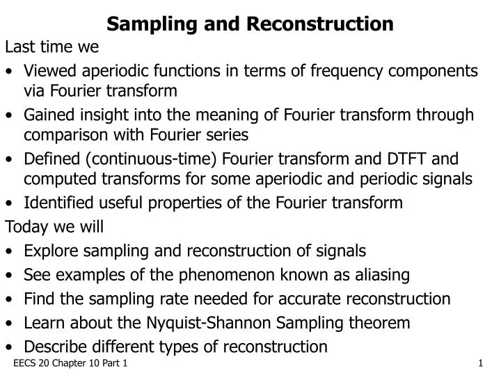
Sampling and Reconstruction Last time we • Viewed aperiodic functions in terms of frequency components via Fourier transform • Gained insight into the meaning of Fourier transform through comparison with Fourier series • Defined (continuous-time) Fourier transform and DTFT and computed transforms for some aperiodic and periodic signals • Identified useful properties of the Fourier transform Today we will • Explore sampling and reconstruction of signals • See examples of the phenomenon known as aliasing • Find the sampling rate needed for accurate reconstruction • Learn about the Nyquist-Shannon Sampling theorem • Describe different types of reconstruction EECS 20 Chapter 10 Part 1
Sampling Let’s define a system called Sampler that converts a continuous-time signal to a discrete-time signal by sampling every T seconds: SamplerT: [RealsComplex][IntegersComplex] x [RealsComplex] and n Integers, SamplerT(x)(n) = x(nT) EECS 20 Chapter 10 Part 1
Sampling Sinusoids: Aliasing Suppose we have a sinusoid with frequency f (in Hertz) that we want to sample. x(t) = cos(2ft+) Sampling the signal at sampling frequency fs = 1/T yields SamplerT(x)(n) = cos(2fnT+) = cos(2n(f/fs)+) Notice that a sinusoid with frequency f′ = f + k fs (k Integers) yields an identical sampled signal! x′(t) = cos(2(f + k fs)t+) SamplerT(x′)(n) = cos(2n(f + k fs)/fs+) = cos(2n(f/fs)+2nk+) = cos(2n(f/fs)+) EECS 20 Chapter 10 Part 1
Aliasing • Thus, when we try to reconstruct a sinusoid from its samples, we can’t know what frequency the original sinusoid had (unless we are given more information). • Every discrete-time signal has many continuous-time “identities”. • We call this phenomenon aliasing. • We want to reconstruct back to the original continuous signal, not an alias of the original signal. • If we have more information about the original signal, e. g., we know that its frequency lies within some range, we may be able to rule out all but one of the aliases. EECS 20 Chapter 10 Part 1
Nyquist Frequency • Suppose we have samples of a sinusoid, and we want to reconstruct the original continuous-time sinusoid. • If we know that the frequency f of the original continuous-time sinusoid lies within the interval [0, ½ fs), then we have ruled out all but one of the possibilities, and have uniquely identified the original signal. • We can accurately reconstruct any continuous-time signal from samples as long as the sampling frequency fs is at least twice as large as the highest frequency component in the original signal. • The frequency ½ fs is known as the Nyquist frequency. It is the highest frequency we can reconstruct from a sampler. EECS 20 Chapter 10 Part 1
Reconstruction There are many different ways to reconstruct a signal. • Zero-order hold: Create the continuous signal x(t) by holding each sample y(n) constant over the time period nT to (n+1)T. • First-order hold: (Linear interpolation) For t between nT and (n+1)T, x(t) varies linearly from x(t)=y(n) at t=nT to x(t)=y(n+1) at t=(n+1)T. • Ideal interpolation: The method that reconstructs sinusoids exactly. We will define this rigorously. Each method of interpolation is itself a system, with domain [IntegersComplex] and range [RealsComplex]. We will now mathematically define each of these systems. EECS 20 Chapter 10 Part 1
Interpolation as Composition of Systems We will represent each method of interpolation as the composition of a special system we will call ImpulseGenT, and another system particular to the method of interpolation. We define the system ImpulseGenT: [IntegersComplex] [RealsComplex] • y [IntegersComplex] and t Reals, The system creates a signal with Dirac delta functions of height y(n) at each time t = nT. Visualize it as a system that turns samples into Dirac delta functions. EECS 20 Chapter 10 Part 1
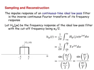
Defining Methods of Interpolation To perform the interpolation, the signal is first sent through ImpulseGenT. The output of ImpulseGenT is then sent through an LTI system that will determine the method of interpolation. For zero-order hold, the LTI system has impulse response For first-order hold (linear interpolation), For ideal interpolation, the impulse response is EECS 20 Chapter 10 Part 1
Nyquist-Shannon Sampling Theorem The ideal interpolation is important because it makes possible the perfect recovery of any signal as long as its highest frequency component is less than the Nyquist frequency. The Nyquist-Shannon Sampling Theorem states: If x is a continuous-time signal with Fourier transform X and if X() is zero outside the range -/T < < /T rad/s, then x = IdealInterpolatorT(SamplerT(x)) where IdealInterpolatorT is the composition of ImpulseGenT and the LTI system defined on the previous slide. EECS 20 Chapter 10 Part 1
Justification for the Sampling Theorem While the formal proof for the theorem is rather technical (you can find it in a DSP book) we will give the intuition behind it: Let’s consider what SamplerT and IdealInterpolatorT do to a signal from a frequency standpoint. The signal x passes through SamplerT first, creating a signal y. Page 437 of the text shows that when a signal is sampled, the old CTFT X and new DTFT Y are related as follows: The CTFT of the original signal is copied and shifted by 2k/T. If the original CTFT is zero outside the interval -/T < < /Tthen the copies won’t overlap! EECS 20 Chapter 10 Part 1
Justification for the Sampling Theorem Now consider what ImpulseGenT does to the sampled signal y. According to page 437 in the text, the Fourier transforms of these two signals are related by Finally, consider what the LTI system does to the signal w. For CTFT EECS 20 Chapter 10 Part 1
Justification for the Sampling Theorem We know that if we pass a signal through an LTI system, the Fourier transform of the output is the product of the Fourier transform of the input and the frequency response. So, the output z of the LTI system has Fourier transform To make Z, we take copies of X, each shifted by 2k/T, and then cut away anything outside of the interval -/T < < /T. Z is the same as X if X() was originally zero outside the interval -/T < < /T. EECS 20 Chapter 10 Part 1