Download
1 / 30
300 likes | 670 Views
Università degli Studi di Genova Corso di Laurea Magistrale in Ingegneria Meccanica Energia & Aeronautica. An experimental setup to investigate intermittency in pipe systems. Relatori: Prof. Alessandro Bottaro Prof. R.I. Sujith. Candidato: Diego Zangrillo. Luglio 2015.

E N D
Università degli Studi di Genova Corso di Laurea Magistrale in Ingegneria Meccanica Energia & Aeronautica An experimental setup to investigate intermittency in pipe systems Relatori: Prof. Alessandro Bottaro Prof. R.I. Sujith Candidato: Diego Zangrillo Luglio 2015
Purpose of the work Investigate Aeroacoustic Intermittency in a very simple experimental setup to understand, predict and avoid it in real systems For example: • In compressor stations of gas transport • In combustor of aircraftengines • In safetyvalves on boilers
Example of events which happened in the past because of Aeroacoustic Instabilities: Oklahoma Gas and Electric Company: safetyvalvesinstalled on boilers The steamdryer in the boiling water reactor (BWR) of QuadCities Unit 2 (QC2) D. Tonon, A. Hirschberg, J. Golliard and S. Ziada, Aeroacoustics of pipe systems with closedbranches, Eindhoven University of Technology, 2010
Experimental Setup Settlingchamber orifice Sampling Time= 30 s Fs= 10 KHz microphone Dimensions: L = 600 mm D = 50 mm d0= 10 mm t = 5 mm Lc = 300 mm dc = 300 mm open end
Data Analysis • Fast Fourier Transform • Hurstexponent • Recurrence Plot • RecurrenceQuantification Analysis
In Orifice Case (A) Re = 3097 Ma = 0.014 Case (B) Re = 4588 Ma = 0.021 Case (C) Re = 4818 Ma = 0.022 Case (D) Re = 5047 Ma = 0.023 Case (A)
In Orifice Case (A) Re = 3097 Ma = 0.014 Case (B) Re = 4588 Ma = 0.021 Case (C) Re = 4818 Ma = 0.022 Case (D) Re = 5047 Ma = 0.023 Case (B)
In Orifice Case (A) Re = 3097 Ma = 0.014 Case (B) Re = 4588 Ma = 0.021 Case (C) Re = 4818 Ma = 0.022 Case (D) Re = 5047 Ma = 0.023 Case (C)
In Orifice Case (A) Re = 3097 Ma = 0.014 Case (B) Re = 4588 Ma = 0.021 Case (C) Re = 4818 Ma = 0.022 Case (D) Re = 5047 Ma = 0.023 Case (D)
HurstExponent The Hurst exponentis used as a measure of long-term memory of time series. It is defined in terms of the asymptotic behaviour of the rescaled range as a function of the time span of a time series as follows: Where: • is the range of the first values, and is their standard deviation • is the expected value • is the time span of the observation (number of data points in a time series) • is a constant. Anti-persistent signal Uncorrelated signal Persistent signal
Recurrence Plot Recurrence is a fundamental property of dynamical systems, which can be exploited to characterise the system’s behaviourin phase space. In 1987, Eckmann et al. introduced the method of recurrence plots (RPs) to visualise the recurrences of dynamical systems. Suppose we have a trajectory of a system in its phase space. The components of these vectors could be, the position and velocity of a pendulum or quantities such as temperature, air pressure, humidity and many others for the atmosphere. The development of the systems is then described by a series of these vectors, representing a trajectory in an abstract mathematical space. Then, the corresponding RP is based on the following recurrence matrix: Where: Number of consideredstates : means equality up to an error (or distance) ε. Ref: N. Marwan, M. Carmen Romano, M. Thiel, J. Kurths, Recurrence plots for the analysis of complex systems, University of Potsdam, 2006
RQA parameters The first recurrence variable is %recurrence rate (%RR). %RRquantifies the percentage of recurrent points falling within the specified radius. This variable can range from 0% (no recurrent points) to 100% (allpointsrecurrent). Ref: C. L. Webber Jr, J. P. Zbilut, Recurrence Quantification Analysis of Nonlinear Dynamical Systems
RQA parameters The second recurrence variable is %determinism (%DET). %DET measures the proportion of recurrent points forming diagonal line structures. Periodic signals will give very long diagonal lines, chaotic signals will give very short diagonal lines, and stochastic signals will give no diagonal lines at all. Ref: C. L. Webber Jr, J. P. Zbilut, Recurrence Quantification Analysis of Nonlinear Dynamical Systems
RQA parameters The third recurrence variable is linemax(LMAX), which is simply the length of the longest diagonal line segment in the plot, excluding the main diagonal line of identity (i = j). Ref: C. L. Webber Jr, J. P. Zbilut, Recurrence Quantification Analysis of Nonlinear Dynamical Systems
Conclusionsand future developments • Intermittencyfound in a simple aeroacoustic system • Need to focus on the first transition • Detection of the intermittencytype
Università degli Studi di Genova Corso di Laurea Magistrale in Ingegneria Meccanica Energia & Aeronautica An experimental setup to investigate intermittency in pipe systems Relatori: Prof. Alessandro Bottaro Prof. R.I. Sujith Candidato: Diego Zangrillo Luglio 2015
RQA parameters The third recurrence variable is %laminarity(%LAM). %LAM isanalogousto %DET except that it measures the percentage of recurrent points comprising vertical line structures rather than diagonal line structures. The line parameter still governs the minimum length of vertical lines to be included.