Download
1 / 24
240 likes | 270 Views
Explore kinship relationships, confounding with QTNs, and statistical power in genomics research. Learn to optimize kinship estimation for accurate genetic analysis.

E N D
Statistical Genomics Lecture 19: SUPER Zhiwu Zhang Washington State University
Outline Kinship based on QTN Confounding between QTN and kinship Complimentary kinship SUPER
More covariates observation mean SNP PC2 u= ] [ ] [ b= b2 b1 b0 Z =X x2 1 x1 y ] [ y = Xb + Zu +e
Variance in MLM y= Xb + Zu + e Var(y)=V=Var(u)+Var(e) Var(u)=G=2K Var(e)=R=I u prediction: Best Linear Unbiased Prediction, BLUP) b prediction: Best Linear Unbiased Estimate, BLUE)
Kinship defined by single marker Sensitive Resistance Adding additional markers bluer the picture
Derivation of kinship QTNs All SNPs Kinship Non-QTNs SNP
Kinship evolution QTNs All traits Pedigree Markers QTNs QTNs Single trait QTNs Remove QTN one at a time Average Realized
Mimic QTN-1 1. Choose t associated SNPs as QTNs each represent an interval of size s. 2. Build kinship from the t QTNs 3. Optimization on t and s 4. For a SNP, remove the QTNs in LD with the SNP, e.g. R square > 1% 5. Use the remaining QTNs to build kinship for testing the SNP
Statistical power of kinship from SUPER (Settlement of kinship Under Progressively Exclusive Relationship) Qishan Wang PLoS One, 2014
Sandwich Algorithm in GAPIT Input KI GP GK GD KI GK CMLM/ MLM/GLM SUPER/ FaST GP Optimization of bin size and number GK KI CMLM/ MLM/GLM SUPER/ FaST GP KI: Kinship of Individual GP: Genotype Probability GD: Genotype Data GK: Genotype for Kinship
#RUN SUPER myGAPIT=GAPIT( Y=mySim$Y, GD=myGD, GM=myGM, QTN.position=mySim$QTN.position, PCA.total=3, sangwich.top="MLM", #options are GLM,MLM,CMLM, FaST and SUPER sangwich.bottom="SUPER",#options are GLM,MLM,CMLM, FaST and SUPER LD=0.1, memo="SUPER") SUPER in GAPIT #GAPIT library('MASS') # required for ginv library(multtest) library(gplots) library(compiler) #required for cmpfun library("scatterplot3d") source("http://www.zzlab.net/GAPIT/emma.txt") source("http://www.zzlab.net/GAPIT/gapit_functions.txt") source("~/Dropbox/GAPIT/Functions/gapit_functions.txt") myGD=read.table(file="http://zzlab.net/GAPIT/data/mdp_numeric.txt",head=T) myGM=read.table(file="http://zzlab.net/GAPIT/data/mdp_SNP_information.txt",head=T) #Siultate 10 QTN on the first chromosomes X=myGD[,-1] index1to5=myGM[,2]<6 X1to5 = X[,index1to5] taxa=myGD[,1] set.seed(99164) GD.candidate=cbind(taxa,X1to5) mySim=GAPIT.Phenotype.Simulation(GD=GD.candidate,GM=myGM[index1to5,],h2=.5,NQTN=10,QTNDist="norm")
GAPIT.FDR.TypeI Function myStat=GAPIT.FDR.TypeI(WS=c(1e0,1e3,1e4,1e5), GM=myGM, seqQTN=mySim$QTN.position, GWAS=myGAPIT$GWAS)
Area Under Curve (AUC) par(mfrow=c(1,2),mar = c(5,2,5,2)) plot(myStat$FDR[,1],myStat$Power,type="b") plot(myStat$TypeI[,1],myStat$Power,type="b")
Replicates nrep=3 set.seed(99164) statRep=replicate(nrep, { mySim=GAPIT.Phenotype.Simulation(GD=GD.candidate,GM=myGM[index1to5,],h2=.5,NQTN=10,QTNDist="norm") myGAPIT=GAPIT( Y=mySim$Y, GD=myGD, GM=myGM, QTN.position=mySim$QTN.position, PCA.total=3, sangwich.top="MLM", #options are GLM,MLM,CMLM, FaST and SUPER sangwich.bottom="SUPER", #options are GLM,MLM,CMLM, FaST and SUPER LD=0.1, memo="SUPER") myStat=GAPIT.FDR.TypeI(WS=c(1e0,1e3,1e4,1e5),GM=myGM,seqQTN=mySim$QTN.position,GWAS=myGAPIT$GWAS) })
Means over replicates power=statRep[[2]] #FDR s.fdr=seq(3,length(statRep),7) fdr=statRep[s.fdr] fdr.mean=Reduce ("+", fdr) / length(fdr) #AUC: power vs. FDR s.auc.fdr=seq(6,length(statRep),7) auc.fdr=statRep[s.auc.fdr] auc.fdr.mean=Reduce ("+", auc.fdr) / length(auc.fdr)
Plots of power vs. FDR theColor=rainbow(4) plot(fdr.mean[,1],power , type="b", col=theColor [1],xlim=c(0,1)) for(i in 2:ncol(fdr.mean)){ lines(fdr.mean[,i], power , type="b", col= theColor [i]) }
Highlight Kinship based on QTN Confounding between QTN and kinship Complimentary kinship SUPER