Download

1 / 58
730 likes | 1.09k Views
Multispectral Imaging and Unmixing. Jürgen Glatz Chair for Biological Imaging www.cbi.ei.tum.de. Munich, 06/06/12. Intraoperative Fluorescence Imaging. Fluorescence Channel. Color Channel . Outline. Multispectral Imaging Unmixing Methods Exercise: Implementation.

E N D
Multispectral Imaging and Unmixing Jürgen Glatz Chair for Biological Imaging www.cbi.ei.tum.de Munich, 06/06/12
Intraoperative Fluorescence Imaging Fluorescence Channel Color Channel
Outline • Multispectral Imaging • Unmixing Methods • Exercise: Implementation
Multispectral Imaging • Multispectral Imaging • Unmixing Methods • Exercise: Implementation
Multispectral Imaging Nature Spectral Resolution Sensitivity Range Spatial Resolution Magnification Technology Multispectral Imaging Spectral Resolution has practically not improved since first camera Spatial Resolution and Magnificationare significantly improved
Color Vision Anyone feeling hungry? Monochrome image of an apple tree Color image of an apple tree • Color vision helps to distinguish and identify objects against their background (here: fruit and foliage) • Color vision provides contrast based on optical properties
Color Vision Spectral sensitivity of the human eye low light short mid long wavelength perception • Color receptors (cone cells) with different spectral sensitivity enable trichromatic vision • Limited spectral range and poor resolution blue green red blue green red blue green red
Limited spectral range Visible Ultraviolet Evening primrose Cleopatra butterfly • Human eyes can only see a portion of the light spectrum (ca. 400-750nm) • Certain patterns are invisible to the eye
Differentchemicalcomposition Same colorappearance Limited spectral resolution chlorophyll plastic • Color vision is insufficient to distinguish between two green objects • Differences in the spectra reveal different chemical composition blue green red blue green red
Optical Spectroscopy • Absorbance • Fluorescence • Transmittance • Emission • Spectroscopy analyzes the interaction between optical radiation and a sample (as a function of λ) • Provides compositional and structural information
Directions of optical Methods Spectroscopy Imaging Currently there are two “directions” in optical analysis of an object A Camera B Spectrometer Provides spatial information Provides spectral information Reveals morphological features No information about structure or composition / no spectral analysis Spectrum reveals composition and structure No information about spatial distribution
Imaging Spectroscopy Imaging Spectroscopy Imaging Spectroscopy Spatial dimension y Spectral dimension λ Spatial information Spectral information Spatial dimension x Spatial dimension y Spectral dimension λ Spatial dimension x Spectral Cube Spatial and spectral information
Spectral Cube Chemicalcompound A Chemicalcompound B Wavelength Pseudo-color image representing the distribution of compounds A and B (chlorophyll and plastic) λ8 Wavelength λ7 λ6 λ5 λ4 λ3 λ2 λ1 • Acquisition of spatially coregistered images at different wavelengths • The maximum number of components that can be distinguished equals the number of spectral bands • The accuracy of spectral unmixing increases with the number of bands
Multispectral Imaging Modalities • Camera + Filter Wheel • Bayer Pattern • Cameras + Prism • Multispectral Optoacoustic Tomography • etc.
Let’s find those apples • Multispectral imaging alone is only one side of the medal • Appropriate data analysis techniques are required to extract information from the measurements
Unmixing Methods • Multispectral Imaging • Unmixing Methods • Exercise: Implementation
The Unmixing Problem Unmixing • Finding the sources that constitute the measurements • For multispectral imaging this means separating image components of different, overlapping spectra • Unmixing is a general problem in (multivariate) data analysis
Multifluorescence Microscopy • Disjoint spectra can be separated by bandpass filtering • Overlapping emission spectra create crosstalk
Autofluorescence I λ • Autofluorescence exhibits a broadband spectrum • Only mixed observations of the components can be measured • Post-processing to unmix them
Forward Modeling What constitutes a multispectral measurement at a certain point and wavelength? Principle of superposition: Sum of individual component emission A component‘s emission over different wavelengths λ is denoted by its spectrum, its spatial distribution is still to be defined.
Setting up a simple forward problem (1) • Two fluorochromes on a homogeneous background • Note: We define images as row vectors of length n • All components are merged in the (n x k) source matrix O n: Number of image pixelsk: Number of spectral components
Setting up a simple forward problem (2) Relative Absorption [%] • Defining the emission spectra for all components at the measurement points • Combining them into the (k x m) spectral matrix Wavelength [nm] k: Number of spectral components m: Number of multispectral measurements m ≥ k
Setting up a simple forward problem (3) Relative Absorption [%] • Two fluorochromes on a homogeneous background • Heavily overlapping spectra • 25 equidistant measurements under ideal conditions Wavelength [nm]
Mathematical Formulation (+N) Multispectral measurement matrix (n x m) Original component matrix (n x k) Spectral mixing matrix (k x m) Noise, artefacts, etc. (n x m)
Mathematical Formulation = • 10000x25 10000x3 3x25
Linear Regression: Spectral Fitting • Reconstructing O • System generally overdetermined: No direct inverse S-1 • Generalized inverse: Moore-Penrose PseudoinvereS+ • Spectral Fitting: Finding the components that best explain the measurements given the spectra • Minimizing the error:
Spectral Fitting • Orthogonality principle: optimal estimation (in a least squares sense) is orthogonal to observation space
Spectral Fitting Spectral Fitting • Given full spectral information (i.e. about all source components) the data can be unmixed
Multifluorescence Imaging RGB image FITC TRITC Cy3.5 Food Nude mice with two different species of autofluorescence and three subcutaneous fluorophore signals: FITC, TRITC and Cy3.5. (Totally 5 signals) Autofluorescence Composite
Spectral Fitting Fast, easy and computationally stable Known order and number of unmixed components Quantitative Requires complete spectral information Crucially depends on accuracy of spectra (systematic errors) Suitable for detection and localization of known compositions
Still no apples… ? ?
Principal Component Analysis • Blind source separation (BSS) technique • Requires no a priori spectral information • Estimates both O and S from M • Assumption:Sources are uncorrelated, while mixed measurements are not
Principal Component Analysis • Unmixing by decorrelation: Orthogonal linear transformation • Transforms the data into a space spanned by the orthogonal PCs • Maximum variance along first PC, maximum remaining variance along second PC, etc.
Unmixing multispectral data with PCA • 25 multispectral measurements are correlated • Their entire variance can (ideally) be expressed by only 3 PCs Dimension reduction • Those 3 PCs are the unmixed sources • Note that matrix orientations may vary between different implementations
Computing PCA Method 1 (preferred for computational reasons) • Subtract mean from multispectral observations • Covariance Matrix: • DiagonalizingCM: Eigenvalue Decomposition • Eigenvectors of CM are the principal components, roots of the eigenvalues are the singular values • Projecting Monto the PCs:
Computing PCA with the SVD Method 2 (not suitable for implementation) • Subtract mean from multispectral observations • Singular Value Decomposition: M = UΣVT • Uis a (m x m) matrix of orthonormal (uncorrelated!) vectors • Projecting Monto those decorrelates the measurements • Singular values in Σdenote how much variance is explained by the respective PC
PCA does more than just unmix Mixing S (UT)-1 = U ≈ S PCA Multispectral data space Original data space • Uis a (non-quantitative) approximation of the PCs spectra • These can be used to verify a components identity • Σis the singular value matrixRelatively small singular values indicate irrelevant components UT
Principal Component Analysis (PCA) Needs no a priori spectral information Also reconstructs spectral properties Significance measurement through singular values Unknown order and number of components Generally not quantitative Crucially depends on uncorrelatedness of the sources Suitable for many compounds and identification of unknown components
Advanced Blind Source Separation • Independent Component Analysis (ICA): assumes statistically independent source components, which is a stronger condition than PCA’s orthogonality • Non-negative Matrix Factorization (NNMF): constraint that all elements must be positive • Commonly computed by iterative optimization of cost functions, gradient descent, etc.
Independent Component Analysis • Assumes and requires independent sources: • Independence is stronger than uncorrelatedness
Independent Component Analysis • Central limit theorem: Sum of non-gaussian variables is more gaussian than the individual variables • Kurtosis measures non-gaussianity: • Maximize kurtosis to find IC • Reconstruction:
Practical Considerations • Noise • Artifacts (from reconstruction, reflections, measurement,…) • Systematic errors (spectra, laser tuning, illumination,…) • Unknown and unwanted components
Exercise: Implementation • Multispectral Imaging • Unmixing Methods • Exercise: Implementation
Forward Problem / Mixing • Define at least 3 non-constant images representing the original components • Plot them and store them in the matrix O • Define an emission spectrum for every component at an appropriate number of measurment points • Plot them and store them in the matrix S • Calculate the measurement matrix as M = OS (and save everything)
Forward Problem / Mixing Relative Absorption [%] Wavelength [nm] O S