Classification

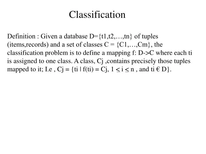
1. Classification Definition : Given a database D={t1,t2,…,tn} of tuples (items,records) and a set of classes C = {C1,…,Cm}, the classification problem is to define a mapping f: D->C where each ti is assigned to one class. A class, Cj ,contains precisely those tuples mapped to it; I.e , Cj = {ti | f(ti) = Cj, 1 < i < n , and ti € D}.

2. Classification problem is implemented in two phases: • Create a specific model by evaluating the training data. This step has input the training data and as output a definition of the model is developed . The model then classifies the training data as accurately as possible. • Apply the model developed in step 1 by classifying tuples from target database.

3. Solution To Problem • Specifying boundaries: • Classification is performed by dividing the input space of potential database tuples into regions where each region is associated with one class. • 2) Using probability distributions: • For any given class , Cj, P(ti|Cj) is PDF for the class evaluated at one point , ti. If a probability of occurrence for each class P(Cj) is known then P(Cj) P(ti|Cj) is used to estimate the probability that ti is in class Cj.

4. 3)Using posterior probabilities: Given a data value ti, we can determine the probability that ti is in class Cj. P(Cj|ti)

5. Issues in Classification: • Missing Data: • Missing data values cause problems during both the training phase and the classification process itself. • It can be handled as : • Ignore the missing data • Assume a value for the missing data • Assume a special value for the missing data.

6. Bayesian Classification: • They are the statistical classifiers. • They can predict class membership probabilities such as probability that a given sample belongs to a particular class. • The naive Bayesian classifier work as follows: • Each data sample is represented by an n-dimensional feature vector, X = {x1,x2,….,xn} , depicting n measurements made on sample from n attributes respectively A1,A2,…,An. • Suppose that there are m classes , C1,C2,..,Cm. Given an unknown data sample X , the classifier will predict that X belongs to the class having the highest posterior probability , conditioned on X. That is , naïve Bayesian classifier assigns an unknown sample X to the class Ci if and only if

7. P(Ci|X) > P(Cj|X) for 1<j<m , j = i Thus we maximize P(Ci|X) . The class Ci for which P(Ci|X) is maximized is called the maximum posteriori hypothesis . By Bayes theorem, P(X|Ci) P(Ci) P(Ci|X) = P(X) 3. P(X) is constant for all classes , only P(X|Ci) P(Ci) is needed to maximized. If the class prior probabilities are not known, then it is commonly assumed that the classes are equally likely, that is, P(C1) = P(C2)= .. = P(Cm) and we would therefore maximize P(X|Ci). Otherwise , we maximize P(X|Ci)P(Ci). Note that the class prior probabilities may be estimated by number of training samples of class Ci.

8. 4. Given data sets with many attributes , it would be extremely computationally expensive to compute P(X|Ci). In order to reduce computation in evaluating P(X|Ci) the naïve assumption of class conditional independence is made. This presumes that the values of the attributes are conditionally independent of one another . Thus , P(X|Ci) = ΠP(xk| Ci) So the probabilities can be estimated from the training samples, where a) If Ak is categorical , then P(xk|Ci) = sik Where sik – number of training samples of class Ci having the value xk for Ak and si – number of training samples belonging to Ci. b) If Ak is continuous – valued , then the attribute is typically assumed to have a Gaussian distribution so that n k=1 si

9. (xk – μCi)2 - P(xk | Ci) = g(xk, μCi , σCi ) = 1 e 2 σCi2 2Π σCi 5. In order to classify an unknown sample X, P(X|Ci)P(Ci) is evaluated for each class Ci. Sample X is then assigned to the class Ci if and only if , P(X|Ci) P(Ci) > P(X|Cj) P(Cj) for 1 < j < m , j = i

10. Distance Based Algorithm Checking the similarity Query to search Engine Web Pages

11. Definition : Given a database D = {t1,t2,..,tn} of tuples where tuple ti = <ti1,ti2,…,tik> contains numeric values and a set of classes C = {C1,C2,…,Cm} where each class Cj = <Cj1,Cj2,…,Cjk> has numeric values , the classification problem is to assign each ti to the Class Cj such that sim(ti,Cj) > sim(ti,Cl) VC1εC2 where Cl = Cj .

12. Algorithm: Input: C1,..,Cm // Centers for each class t // Input tuple to classify Output: c // Class to which t is assigned Simple distance based algorithm dist =  ; for i := 1 to m do if dis(ci,t) < dist , then c = i ; dist = dist(ci,t);

13. K Nearest Neighbors Algorithm: Input: T // training data K // Number of neighbors t // Input tuple to classify Output: c // Class to which t is assigned KNN Algorithm: // to classify tuple using KNN N = 0; // Find set of neighbors , N, for t For each dT do

14. if |N| < K , then N = N U {d} ; else if  u  N such that sim(t,u) < sim(t,d) , then begin N = N – {u}; N = N U {d}; end // Find class for classification c = class to which the most u N are classified;

15. Example: By using previous example , the output classification as training set o/p value , we classify the tuple <Tina,F,1.6>. Suppose that K = 5 given. We then have that the K nearest neighbors to the input tuple are {<Ina,F,1.6>,<Mina,F,1.6>, <Diga,F,1.7>,<Anil,M.1.7>,<leena,F,1.75>}. Among 5 , 4 are Classified as short and one as medium. Thus , the KNN will classify Tina as short.

16. Decision Tree Based Algorithms • The decision tree approach is most useful in classification problems. There are two basic steps in this technique: • Building a tree • Applying a tree • Definition : Given a database D = {t1,t2,..,tn} where ti = <ti1,..,tih> and the database schema contains the following attributes{A1,A2,..,Ah}.Also given is a set of classes C = {C1,..,Cm}. A decision tree or classification tree is a tree associated with D that has the following properties: • Each internal node is labeled with an attribute, Ai. • Each arc is labeled with a predicate that can be applied to the attribute associated with parent. • Each leaf node is labeled with a class , Cj.

17. Height a)Balanced Tree Gender < 1.3m > 2 m =F = M Short Tall Gender Height Height =F =M < 1.3m > 1.8 m > 2 m < 1.5m Height Height Short Medium Tall Short Medium Tall <= 1.8 m <= 1.8 m >= 1.5 m < 1.5 m Height Short Medium Medium Tall < 1.3m > 2 m b)Deep Tree >=1.5m <=18m >1.8m >2m >=1.3m <1.5m Height Medium Gender Tall Short Gender > =2 m < =1.5m =F = M =F = M Tall Short Tall Short Medium Medium Medium c)Bushy Tree d)No gender attributes

18. Factors affecting the DT algorithms • Choosing splitting attributes: • Ordering of splitting attributes: • Splits: • Tree Structure: • Stopping criteria: • Training data: • Pruning:

19. ID3 • ID3 uses a tree representation for concepts. • By choosing a random subset training instances called windows. • Procedure builds a decision tree that correctly classifies all instances in the window . • Tree is then tested on the training instances outside the window. • Once all the instances are classified correctly , then the procedure halts. • Else it adds some of the instances incorrectly classified to the window and repeat the process. • ID3 selects the feature which minimizes the entropy function and thus best discriminates among the instances.

20. ID3 Algorithm • Select a random subset W(window) from the training set. • Build a decision tree for the current window: • Select the best feature which minimizes the entropy function H: • H =  - pi log pi • Where pi – probability associated with ith class , for feature the entropy is calculated for each value. The sum of the entropy weighted by he probability of each value is the entropy for that feature. • Categorizing training instances into subsets by this feature. • Repeat this process recursively until each subset contains instances of one kind or some statistical criterion is satisfied. i

21. 3. Scan the entire training set for exceptions to the decision tree. 4. If exception are found , insert some of them into W and repeat from step 2 . The insertion may be done either by replacing it with the new exceptions. Example : Use the ID3 algorithm to build a decision tree for classifying the following objects:

22. First , we calculate the entropy for each attribute: Size H: = 1/6 ( - 1 log 1) + 4/6 (-2/4 log 2/4) + 1/6(-log 1) = 0.462 Color H: = 3/6 (-2/3 log 2/3 – 1/3 log 1/3) + 3/6(-3/3 log 3/3)=0.318 Surface H: = 5/6(-3/5 log 3/5 – 2/5 log 2/5) + 1/6(-1log1) = )= 0.56 Thus we select the attribute Color as the first decision node since it is associated with the minimum entropy. This node has two branches: Red and Yellow.Under the branch Red, only class A objects fall and hence no further discrimination is needed. Under the branch Yellow we need another attribute to make further distinctions. So we calculate the entropy for the other two attributes under this branch: Size: H = 1/3 (-1 log 1) + 2/3(-2/3 log 1) = 0 Surface H = 3/3(-2/3 log 2/3 – 1/3) = 0.636

23. Color Red Yellow A Size Medium Small A B