Download
1 / 25
250 likes | 261 Views
Status of the BRAMS network and recent progress. H. Lamy & BRAMS team. BRAMS network : full inspection during summer / fall 2018. 26 active Rx 1 Tx. We solved many small (and not so small) problems. Receiving stations. Some problems encountered. Calibrator unplugged

E N D
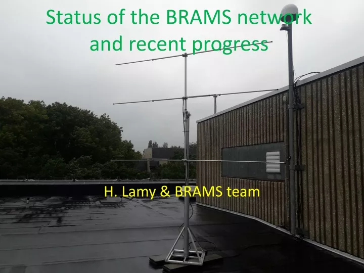
Status of the BRAMS network and recent progress H. Lamy & BRAMS team
BRAMS network : full inspection during summer / fall 2018 • 26 active Rx • 1 Tx We solved many small (and not so small) problems
Receiving stations Some problems encountered • Calibrator unplugged • Meinberg not using GPS NMEA to synchronize the PC Clock • ICOM-R75 not using PRE-AMP2, AGC OFF or using additional functions • ….
Receiving stations : vertical orientation BELEUZ Radiation pattern much more closer to theoretical one BEOVER
Receiving stations : change of azimut orientation Goal : trying to minimize local interference BEREDU
Receiving stations : impedancematching • Mounting specifications of the antenna manual provided at best a return loss S11 -15 dB at f = 49.97 MHz (for most antennas it was lower) and a dip for S11 which was never at 50 MHz but more at f 50.6 – 50.7 MHz • Tests in June with an antenna in Uccle to increase the length of elements by a few cm to decrease the resonance frequency of the antenna. Increase by 3 cm on each side of the 3 elements provides the best results • Length of the matching element chosen to maximize the dip.
ICOM-R75 receivers • 18of them had problems with a progressive loss of sensitivity. • The origin of the problem was identified by M. Anciaux who was able to repair 13 of them • ICOM-R75 are not commercially produced anymore search for new solutions using SDR receivers (see next talk)
Transmitter in Dourbes P 150 W Circular polarisation f = 49.97 MHZ Is this correct? full characterization on 21 September
Transmitter in Dourbes Picotest G5100A Waveform generator Tomco BT00400-AlphaSA-CW Ecoflex 15 RF cable
Transmitter in Dourbes • Full characterization of the Tx on 21/09/2018 usingdummyload, wattmeter, oscilloscope and antennaanalyzer • Power amplifier characterization: using the Wattmeter in between the amplifier and the antenna, wefoundP_forward 110 W and P_reflected 15 W, providing a SWR 2.2. Total power at the antennashouldthenbe of the order of 95 W. More accuratemeasurementsusing the dummyload and the oscilloscope giveP_forward = 104.7 W incident on the antennacable. • Antennacharacterization: Two 50 cables in parallellinked by a T equivalentresistance (resistive part) measured at the extremity of the RF cableis 25.6 as expected. Takingintoaccount the losses in the cable, weexpect an incident power of 95.5 W at the entrance of the T • Independent measurements of the adaptation of the twoindividualantennas: SWR=1.68 and 1.16 • Ant 1 : P=44.3 W – Ant 2 : P=40.6 W, = -96°
Transmitter in Dourbes • Conclusions : • Weemit far lessthan 150 Watts ( 90 Watts) • The emittedwaveis not perfectlycircularlypolarized but not too far (96° instead of 90°) • Still to do : • Measurements of the radiation pattern in-situ usingour drone (March?) • Replacement of the current system with an improved design to guarantee 150 W emission and perfectlycircularlypolarizedwave
Data transfer • Data from all 26 stations are now transferred via FTP • 23 stations are automatically transferring the data daily using the BRAMS-FTP facility • 3 stations are sending their data weekly using FileZilla • 20 stations can be accessed remotely via Team Viewer or Remote Desktop. BRAMS availability tool
Quality check of the data • Matlab and/or Python tools have been developed to • Check for saturation • Derive the amplitude and exact frequency of the calibrator • Amplitude provides an estimate of the response of the front-end of the receiving station (ICOM R-75 + sound-card) • Frequencyprovides an estimate of the frequency offset due to the poorstability of the LO of the ICOM-R75 • Thesetools are currentlybeingimplemented to the archiving system in order to quicklyidentifypotentialproblems (mostlywith the receiver but alsocalibrator off, etc …)
Saturation of the data Total nb of samples in a WAV file 5512 * 300 1 653 600 01H30 07H10
Saturation of the data 01H30 07H10
Amplitude and frequency of the calibrator signal • First wetake the FFT of the whole 5 minutes long WAV file (ffs/nfft = 1/300 Hz) • Wethenaccuratelydetermine the frequency and amplitude of the calibrator signal. Twodifferent techniques have been used • Fit a sincfunction to the FFT spectrum in the region of the calibratorfrequency • « Integrate » the contributions of the various FFT frequencies in a limited range of frequencies and subtract an estimate of the local noise
Method 1 : sinc fit of the FFT spectrum Works well in Humain FFT values FFT Frequency Red discrete crosses = FFT values Blue continuous curve = sinc fit
Method 2 : « integration » of the FFT spectrum contributions The LO of the ICOM-R75 is not stabilized. Instead we locate the max of the FFT spectrum and sum the values of the FFT spectrum in a small frequency range centered on it Then we estimate the contribution of the noise in a frequency range nearby and subtract it Based on Parseval’s theorem :
Utility of the amplitude of the calibrator signal • To detect a potential problem with the ICOM-R75 (progressive decrease of amplitude over a period of time) • To calibrate power measurements of meteor echoes in Watts (see talk about CAMS/BRAMS comparisons)