Download
1 / 39
400 likes | 586 Views
Chapter. The Normal Probability Distribution. THIS CHAPTER’S GOALS. TO LIST THE CHARACTERISTICS OF THE NORMAL DISTRIBUTION. TO DEFINE AND CALCULATE Z VALUES. TO DETERMINE PROBABILITIES ASSOCIATED WITH THE STANDARD NORMAL DISTRIBUTION.

E N D
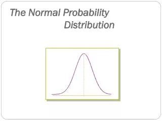
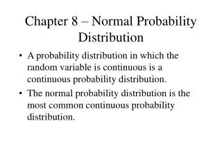
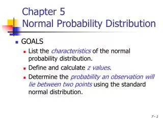
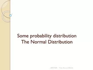
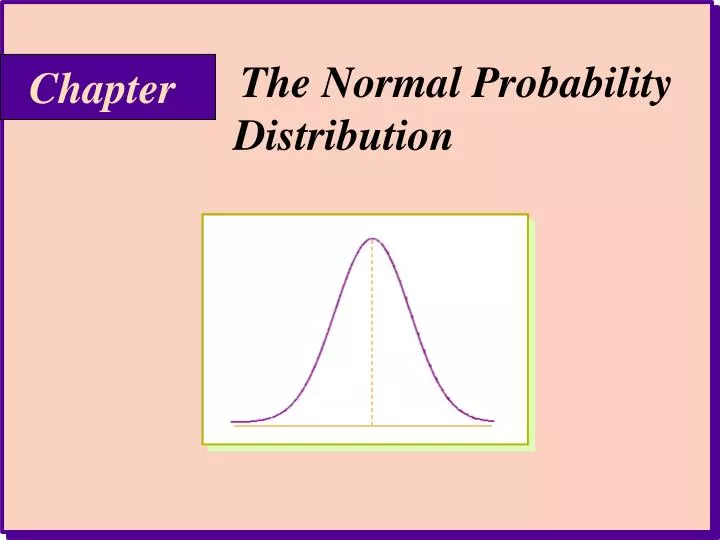
Chapter The Normal Probability Distribution
THIS CHAPTER’S GOALS • TO LIST THE CHARACTERISTICS OF THE NORMAL DISTRIBUTION. • TO DEFINE AND CALCULATE Z VALUES. • TO DETERMINE PROBABILITIES ASSOCIATED WITH THE STANDARD NORMAL DISTRIBUTION. • TO USE THE NORMAL DISTRIBUTION TO APPROXIMATE THE BINOMIAL DISTRIBUTION.
CHARACTERISTICS OF A NORMAL PROBABILITY DISTRIBUTION • The normal curve isbell-shapedand has a single peak at the exact center of the distribution. • The arithmetic mean, median, and mode of the distribution are equal and located at the peak. • Half the area under the curve is above this center point, and the other half is below it. • The normal probability distribution is symmetrical about its mean. • It is asymptotic - the curve gets closer and closer to the x-axis but never actually touches it.
CHARACTERISTICS OF A NORMAL DISTRIBUTION Normal curve is symmetrical - two halves identical - Tail Tail 0.5 0.5 Theoretically, curve extends to - infinity Theoretically, curve extends to + infinity Mean, median, and mode are equal
Normal Distributions with Equal Means but Different Standard Deviations. s = 3.1 s = 3.9 s = 5.0 m = 20
Normal Probability Distributions with Different Means and Standard Deviations. m = 5, s = 3 m = 9, s = 6 m = 14, s = 10
THE STANDARD NORMAL PROBABILITY DISTRIBUTION • A normal distribution with a mean of 0 and a standard deviation of 1 is called the standard normal distribution. • z value:The distance between a selected value, designated X, and the population mean m, divided by the population standard deviation, s. • The z-value is the number of standard deviations X is from the mean.
EXAMPLE • The monthly incomes of recent MBA graduates in a large corporation are normally distributed with a mean of $2,000 and a standard deviation of $200. What is the z value for an income X of $2,200? $1,700? • For X = $2,200 and since z = (X - m)/s, then z = (2,200 - 2,000)/200 = 1. • Az value of 1 indicates that the value of $2,200 is 1 standard deviationabovethe mean of $2,000.
EXAMPLE (continued) • For X = $1,700 and since z = (X - m)/s, then z = (1,700 - 2,000)/200 = -1.5. • Az value of -1.5 indicates that the value of $2,200 is 1.5 standard deviation below the mean of $2,000. • How might a corporation use this type of information?
AREAS UNDER THE NORMAL CURVE • About 68 percent of the area under the normal curve is within plus one and minus one standard deviation of the mean. This can be written as m ± 1s. • About 95 percent of the area under the normal curve is within plus and minus two standard deviations of the mean, written m ± 2s. • Practically all (99.74 percent) of the area under the normal curve is within three standard deviations of the mean, written m ± 3s.
Between: 1. 68.26% 2. 95.44% 3. 99.97% m+3s m-2s m-1s m m+1s m+2s m+3s
P(z)=? • A typical need is to determine the probability of a z-value being greater than or less than some value. • Tabular Lookup (Appendix D, page 474) • EXCEL Function =NORMSDIST(z)
EXAMPLE • The daily water usage per person in Toledo, Ohio is normally distributed with a mean of 20 gallons and a standard deviation of 5 gallons. • About 68% of the daily water usage per person in Toledo lies between what two values?
EXAMPLE • The daily water usage per person in Toledo (X), Ohio is normally distributed with a mean of 20 gallons and a standard deviation of 5 gallons. • What is the probability that a person selected at random will use less than 20 gallons per day? • What is the probability that a person selected at random will use more than 20 gallons per day?
EXAMPLE (continued) • What percent uses between 20 and 24 gallons? • The z value associated with X = 20 isz= 0 and with X = 24, z = (24 - 20)/5 = 0.8 P(20 < X < 24) = P(0 < z < 0.8) = 0.2881=28.81% • What percent uses between 16 and 20 gallons?
EXAMPLE (continued) • What is the probability that a person selected at random uses more than 28 gallons?
P(z > 1.6) = 0.5 - 0.4452 = 0.0048 Area = 0.4452 z 1.6
EXAMPLE (continued) • What percent uses between 18 and 26 gallons?
Total area = 0.1554 + 0.3849 = 0.5403 Area = 0.1554 Area = 0.3849 z - .4 1.2
EXAMPLE (continued) • How many gallons or more do the top 10% of the population use? • Let X be the least amount. Then we need to find Y such that P(X ³Y) = 0.1 To find the corresponding z value look in the body of the table for (0.5 - 0.1) = 0.4. The corresponding z value is 1.28 Thus we have (Y - 20)/5 = 1.28, from which Y= 26.4. That is, 10% of the population will be usingat least 26.4 gallons daily.
(Y - 20)/5 = 1.28 Y= 26.4 0.4 0.1 z 1.28
EXAMPLE • A professor has determined that the final averages in his statistics course is normally distributed with a mean of 72 and a standard deviation of 5. He decides to assign his grades for his current course such that the top 15% of the students receive an A. What is the lowest average a student must receive to earn an A?
(Y - 72)/5 = 1.04 Y = 77.2 0.35 0.15 z 1.04
EXAMPLE • The amount of tip the waiters in an exclusive restaurant receive per shift is normally distributed with a mean of $80 and a standard deviation of $10. A waiter feels he has provided poor service if his total tip for the shift is less than $65. Based on his theory, what is the probability that he has provided poor service?
Area = 0.5 - 0.4332 = 0.0668 Area = 0.4332 z - 1.5
THE NORMAL APPROXIMATION TO THE BINOMIAL • Using the normal distribution (a continuous distribution) as a substitute for a binomial distribution (a discrete distribution) for large values of n seems reasonable because as nincreases, a binomial distribution gets closer and closer to a normal distribution. • When to use the normal approximation? • The normal probability distribution is generally deemed a good approximation to the binomial probability distribution when np and n(1 - p)are both greater than 5.
Binomial Distribution with n = 3 and p = 0.5. P(r) 0.5 0.4 0.3 0.25 r 0 1 2
Binomial Distribution with n = 20 and p = 0.5. P(r) Observe the Normal shape. r
THE NORMAL APPROXIMATION (continued) • Recall for the binomial experiment: • There are only two mutually exclusive outcomes (success or failure) on each trial. • A binomial distribution results from counting the number of successes. • Each trial is independent. • The probability p is fixed from trial to trial, and the number of trials n is also fixed.
CONTINUITY CORRECTION FACTOR • The value 0.5 subtracted or added, depending on the problem, to a selected value when a binomial probability distribution, which is a discrete probability distribution, is being approximated by a continuous probability distribution--the normal distribution. • The basic concept is that a slice of the normal curve from x-0.5 to x+0.5 is approximately equal to P(x).
EXAMPLE • A recent study by a marketing research firm showed that 15% of the homes had a video recorder for recording TV programs. A sample of 200 homes is obtained. (Let X be the number of homes). • Of the 200 homes sampled how many would you expect to have video recorders? • m = np (0.15)(200) = 30 & n(1 - p) = 170 • What is the variance? • s2 = np(1 - p) = (30)(1- 0.15) = 25.5
EXAMPLE (continued) • What is the standard deviation? • s = Ö(25.5) = 5.0498. • What is the probability that less than 40 homes in the sample have video recorders? • We need P(X < 40) = P(X £ 39). So, using the normal approximation, P(X £ 39.5) » P[z£ (39.5 - 30)/5.0498] = P(z£ 1.8812) » P(z £ 1.88) = 0.5 + 0.4699 = 0.9699 Why did I use 39.5 ? ... How would you calculate P(X=39) ?
P(z £ 1.88) = 0.5 + 0.4699 = 0.9699 0.5 0.4699 z 1.88
EXAMPLE (continued) • What is the probability that more than 24 homes in the sample have video recorders?
P(z ³ -1.09) = 0.5 + 0.3621 = 0.8621. 0.5 0.3621 z -1.09
EXAMPLE (continued) • What is the probability that exactly 40 homes in the sample have video recorders?
P(1.88 £ z £ 2.08)= 0.4812 - 0.4699 = 0.0113 1.88 2.08 0.4699 0.4812 z