Download

1 / 88
880 likes | 1.25k Views
3. 7. Chapter The Normal Probability Distribution. © 2010 Pearson Prentice Hall. All rights reserved. Section 7.1 Properties of the Normal Distribution. EXAMPLE Illustrating the Uniform Distribution.

E N D
3 7 Chapter The Normal Probability Distribution © 2010 Pearson Prentice Hall. All rights reserved
Section 7.1 Properties of the Normal Distribution © 2010 Pearson Prentice Hall. All rights reserved
EXAMPLE Illustrating the Uniform Distribution Suppose that United Parcel Service is supposed to deliver a package to your front door and the arrival time is somewhere between 10 am and 11 am. Let the random variable X represent the time from10 am when the delivery is supposed to take place. The delivery could be at 10 am (x = 0) or at 11 am (x = 60) with all 1-minute interval of times between x = 0 and x = 60 equally likely. That is to say your package is just as likely to arrive between 10:15 and 10:16 as it is to arrive between 10:40 and 10:41. The random variable X can be any value in the interval from 0 to 60, that is, 0 <X< 60. Because any two intervals of equal length between 0 and 60, inclusive, are equally likely, the random variable X is said to follow a uniform probability distribution.
The graph below illustrates the properties for the “time” example. Notice the area of the rectangle is one and the graph is greater than or equal to zero for all x between 0 and 60, inclusive. Because the area of a rectangle is height times width, and the width of the rectangle is 60, the height must be 1/60.
Values of the random variable X less than 0 or greater than 60 are impossible, thus the equation must be zero for X less than 0 or greater than 60.
The area under the graph of the density function over an interval represents the probability of observing a value of the random variable in that interval.
EXAMPLE Area as a Probability The probability of choosing a time that is between 15 and 30 seconds after the minute is the area under the uniform density function. Area = P(15 <x< 30) = 15/60 = 0.25 15 30
A probability density function (a) Shows the number of observations for a variable (b) Lists the probabilities for a discrete random variable (c) Shows how dense the mean and standard deviation are compared to the median (d) Is used to compute probabilities for continuous random variables (e) Not sure
True or False: The area under a probability density function must equal 1.
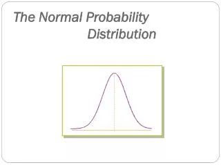
Relative frequency histograms that are symmetric and bell-shaped are said to have the shape of a normal curve.
If a continuous random variable is normally distributed, or has a normal probability distribution, then a relative frequency histogram of the random variable has the shape of a normal curve (bell-shaped and symmetric).
The curve below is not a normal curve because (a) It is skewed left (b) It is not continuous (c) It is skewed right (d) It has outliers (e) Not sure
What is the mean of the normal distribution shown? (a) 120 (b) 20 (c) 140 (d) 100 (e) Not sure
Each graph represents a normal curve with mean μ = 100. Which graph indicates the normal random variable X has more dispersion? (a) Blue graph (b) Red graph (c) Not sure
The normal density curve (a) Is not symmetric (b) Has an area under the curve equal to one. (c) Always has a mean of 0 (d) Has positive and negative values (e) Not sure
EXAMPLE A Normal Random Variable The data on the next slide represent the heights (in inches) of a random sample of 50 two-year old males. (a) Draw a histogram of the data using a lower class limit of the first class equal to 31.5 and a class width of 1. (b) Do you think that the variable “height of 2-year old males” is normally distributed?
36.0 36.2 34.8 36.0 34.6 38.4 35.4 36.8 34.7 33.4 37.4 38.2 31.5 37.7 36.9 34.0 34.4 35.7 37.9 39.3 34.0 36.9 35.1 37.0 33.2 36.1 35.2 35.6 33.0 36.8 33.5 35.0 35.1 35.2 34.4 36.7 36.0 36.0 35.7 35.7 38.3 33.6 39.8 37.0 37.2 34.8 35.7 38.9 37.2 39.3
In the next slide, we have a normal density curve drawn over the histogram. How does the area of the rectangle corresponding to a height between 34.5 and 35.5 inches relate to the area under the curve between these two heights?
EXAMPLE Interpreting the Area Under a Normal Curve • The weights of giraffes are approximately normally distributed with mean μ = 2200 pounds and standard deviation σ = 200 pounds. • Draw a normal curve with the parameters labeled. • Shade the area under the normal curve to the left of x = 2100 pounds. • Suppose that the area under the normal curve to the left of x = 2100 pounds is 0.3085. Provide two interpretations of this result. (a), (b) • (c) • The proportion of giraffes whose weight is less than 2100 pounds is 0.3085 • The probability that a randomly selected giraffe weighs less than 2100 pounds is 0.3085.
EXAMPLE Relation Between a Normal Random Variable and a Standard Normal Random Variable The weights of giraffes are approximately normally distributed with mean μ = 2200 pounds and standard deviation σ = 200 pounds. Draw a graph that demonstrates the area under the normal curve between 2000 and 2300 pounds is equal to the area under the standard normal curve between the Z-scores of 2000 and 2300 pounds.
The area to the right of 0 under the standard normal curve is equal to (a) 0.0 (b) 0.25 (c) 0.5 (d) 1.0 (e) Not sure
If the area to the right of 0.41 under the standard normal curve is equal to 0.34, then the area to the left of 0.41 is equal to (a) 0.66 (b) 0.50 (c) 0.34 (d) 0.17 (e) Not sure
The table gives the area under the standard normal curve for values to the left of a specified Z-score, zo, as shown in the figure.
EXAMPLE Finding the Area Under the Standard Normal Curve Find the area under the standard normal curve to the left of z = -0.38. Area left of z = -0.38 is 0.3520.
Find the area under the standard normal curve to the left of z = 1.54.
Area under the normal curve to the right of zo =1 – Area to the left of zo
EXAMPLE Finding the Area Under the Standard Normal Curve Find the area under the standard normal curve to the right of Z = 1.25. Area right of 1.25 = 1 – area left of 1.25 = 1 – 0.8944 = 0.1056
Find the area under the standard normal curve to the right of z = -2.38.
EXAMPLE Finding the Area Under the Standard Normal Curve Find the area under the standard normal curve between z = -1.02 and z = 2.94. • Area between -1.02 and 2.94 = (Area left of z = 2.94) – (area left of z = -1.02) • = 0.9984 – 0.1539 • = 0.8445