Download
1 / 1
10 likes | 154 Views
Seasonal Variation of Boundary Layer Carbon Monoxide Dispersion over Norman, Oklahoma using the AERMOD Model. Jeremy Halland December 13, 2006. Background and Purpose:. Spring Study: March 11-14, 2006. --- Forced BL - - Convective BL.

E N D
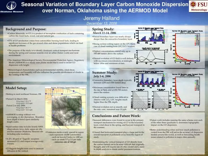
Seasonal Variation of Boundary Layer Carbon Monoxide Dispersion over Norman, Oklahoma using the AERMOD Model Jeremy Halland December 13, 2006 Background and Purpose: Spring Study: March 11-14, 2006 --- Forced BL - - Convective BL • Carbon Monoxide, or CO, is a product of incomplete combustion of fuels containing • carbon like fossil fuels, wood, coal and natural gas. • 77% of CO production comes from automobiles burning fossil fuels, leading to • significant increases of the gas around cities and dense populations which can lead • to health problems. • The purpose of the study is to identify dominant vertical transport mechanisms • during the spring and summer seasons over an urban (future work) and rural • environment. • The American Meteorological Society/Environmental Protection Agency Regulatory • Model (AERMOD) is a steady state plume model that is used to model CO • dispersion with height. • Meteorological characteristics such as environmental stability, wind shear, • temperature and humidity will also influence the possible involvement of clouds in • the venting of the PBL. • Forced boundary layer was nearly always • deeper than the convective boundary layer. • Strong cyclone exiting region on the 13th, likely • case of cloud venting from LFC/LCL location. • Highest concentrations extend only up to • 350-400 meters above the surface. • Diurnal evolution of CO field is well defined, • with maximum concentrations at midnight • below 100m and minimum at 6am. Summer Study: July 1-6, 2006 --- Forced BL - - Convective BL • Convective boundary layer depth typically • between 1250 and 1500 meters deep. • Maximum concentration found later in • the day at 9pm, and at 650-700 meters • above the surface. • Cloud venting scenario was difficult to • observe with LCL/LFC heights much • higher than the PBL depth. • Diurnal evolution not as smooth, and • the min. conc. remained near 10 ppb. Model Setup: • Setting in rural northeast Norman, OK • Period 1 in March 2006: • Avg temp = 55.1 °F • Avg wind = 13.5 mph • Period 2 in July 2006: • Avg temp = 86.2 °F • Avg wind = 10.3 mph • AERMOD is setup without wet- • scavenging, or dry-deposition. Boundary • layer depth is based upon similarity • length scales. • Input surface data includes hourly NWS • observations, twice daily upper-air obs, • and five-minute Oklahoma Mesonet obs • including solar insolation. • A 25 x 40 grid of ‘flagpole’ receptors • measured CO, and output average every • 3 hours. • 22 flagpole heights were used to measure • diffusion in the vertical. Temperature (°C) Temperature (°C) Conclusions and Future Work: • Seasonal differences were found to occur in the primary • transport mechanism for mixing of CO in the boundary • layer, wind shear in the spring, and buoyant transport in • the summer. • I found that horizontal transport plays a large part in the • overall transport of pollutants away from the region of • study. • Determining the vertical transport of CO directly from • the surface turned out to be more difficult that originally • thought, and will require use of a flux model and a more • in depth analysis to obtain useful parameterizations. • Future work includes running the same scheme over each • of the other three quadrants to determine topographic • impact on the CO dispersion. • Better understanding when and how much pollution is • vented from the PBL will aid in the accuracy of dispersion • models around the world, as well as forecasting health • issues related to pollution in major cities annually. • 9 emission stacks evenly spaced in region • - each represents 10,000 automobiles • - each car travels 5 miles in 1200 sec. • - each car emits 3.5 g CO per mile • - emission rate of 142 g/s