Download
1 / 34
340 likes | 695 Views
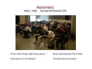
VLBI Astrometry Mark J. Reid Harvard-Smithsonian CfA. VLBI Astrometry Mark J. Reid Harvard-Smithsonian CfA. “From little things, big things grow…” Bruce Springsteen/Paul Kelly. Calibrator. Where is the Galactic Center?. Sun. Harlow Shapley (ca. 1920). Galactic Center.

E N D
VLBI AstrometryMark J. ReidHarvard-Smithsonian CfA “From little things, big things grow…” Bruce Springsteen/Paul Kelly Calibrator
Where is the Galactic Center? Sun Harlow Shapley (ca. 1920) Galactic Center Globular clusters based on Cepheid distances Projected onto Galactic Plane
Galactic Center Stellar Orbits VLT: 2 mm • M = 4 x 10⁶ Msun • R < 50 AU • Den. > 1017 Msun/pc3 5” Genzel et al / Ghez et al 0.04” What can radio observations tell us?...
Where is the Galactic Center? VLA l = 6 cm 1.3 cm 5” Zhao Jun-Hui Sgr A*
Sgr A* Proper Motion IR Stellar Orbits: MIR ~ 4 x 10⁶ Msun R < 50 AU Radio Observations: Sgr A* motionless M > 10% of MIR Observed size: R < 0.5 AU IR + Radio data combined: Dark mass = luminous source Density > 1022 Msun/pc3 Overwhelming evidence for a Super-Massive Black Hole Best Fit Gal. Plane Vsun NGP How do we make such measurements?
Fringe spacing: qf~l/D ~ 1 cm / 8000 km = 250 mas Centroid Precision: 0.5 qf / SNR ~ 10 mas Systematics: path length errors ~ 2 cm (~2 l) shift position by ~ 2qf Relative positions (to QSOs): DQ ~ 1 deg (0.02 rad) cancel systematics: DQ*2qf ~ 10 mas Micro-arcsec Astrometry with the VLBA Comparableto GAIA & SIM
(will explain formula later) Note: sq independent of l, since FWHM ~ l/D
Atmospheric & Ionospheric Errors Frequency (maser) Un-modeled Zenith Path Length Atmosphere Ionosphere 43 GHz (SiO) 5 cm 0.5 cm 22 (H2O) 5 2 12 (CH3OH) 5 6 6.7 (CH3OH) 5 20 1.6 (OH) 5 300
DZA ZA
Typical Observing Sequence Source rising Source setting 40 min Time Electronic Cal Phase-ref obs Atmospheric Cal Can share time between two target/reference pairs (within ~1 hour of R.A.) QSO-1(ZA=100), QSO-2(ZA=500), … QSO-15(ZA=300)
Atmospheric Delay Calibration • Measure zenith delay (t0) above each antenna • Spread observing bands to cover 500 MHz st ~ (1/BW) * (1/SNR) • Observe QSOs over range of elevations • Fit to atmospheric model: t0 ~ 0.5 cm accuracy Data Model Residuals
Position Errors DZA Effects of position error of phase reference source: • 1st order correction: position shift of Target • 2nd order corrections: small shift of Target distorts image ZA Target Reference DQ = 1 degree Reference pos. err sq = 0.1 arcsec
Position Errors 2nd order phases Image distortion Effects of position error of phase reference source: • 1st order correction: position shift of Target • 2nd order corrections: small shift of Target distorts image Fitted position shift Target Reference DQ = 1 degree Reference pos. err sq = 0.1 arcsec Need reference position accurate to ~10 mas
Maser as Reference Source Spread over ~ 1” Don’t know which spot to use before getting data What to do…
Reference Source Position Measure with VLBI (need ICRF quasar within about 3 degrees on sky) Measure with VLA (need largest configuration) Use “raw” VLBI data Fringe rate map Invert raw data (Dirty Map)
Calibration: Step 1 • Fix phase errors in VLBA correlator model: • Parallactic Angle (feed rotation effect) CLCOR • Atmospheric zenith delays (“geodetic” blocks) DELZN/CLCOR • Ionospheric zenith delays (global electron models) TECOR • Earth’s Orientation Parameter errors CLCOR • Source coordinate errors (if known) CLCOR
Calibration: Step 2 • Calibrate amplitudes (correlation coefficient flux density): • Correct for clipper bias CLCAL • Apply system temperatures/gain curves APCAL/CLCAL
Calibration: Step 3 • Align electronic phase shifts among bands: • Determine band phases on strong source FRING • Correct all data CLCAL • Fix spectral drift (Doppler shift from Earth’s rotation) • Apply bandpass corrections (if necessary) BPASS • Fourier transform to delays, • Apply phase-slope across delay function, • Inverse Fourier transform back CVEL
Calibration: Step 4 • Phase reference data to 1 source / band / spectral channel: • Calculate phase reference CALIB or FRING • Apply phases to all data CLCAL
Lunar Parallax 7000 km baseline Hipparchus (189 BC) Pete Lawrence’s Digitalsky: http://www.digitalsky.org.uk
Trigonometric Parallax 1 AU • Triangulation using Earth’s orbit as one leg of triangle • Bessel in 1830s measured first accurate stellar distance this way • VLBA accuracy 10 micro-arcsec ! • 10,000x better than Bessel • With such “vision”, could read this from the Moon! D p
Orion Nebular Cluster Parallax D = 414 +/- 7 pc How to fit data & optimize observations? Menten, Reid, Forbrich & Brunthaler (2007)
M M = N
sp = 1 / sqrt( S cos2 wt ) • N = 5 • sp = 1 / sqrt( 2 ) = 0.7 • N = 5 • sp = 1 / sqrt( 3 ) = 0.6 • N = 4 • sp = 1 / sqrt( 4 ) = 0.5
Peculiar Motions of Star Forming Regions • Trace Spiral Arms • In rotating frame seeclear systematic motions: • SFRs orbit galaxy slower than galaxy spins