Download
1 / 71
910 likes | 1.7k Views
Control Systems. Lect.4 Time Response Basil Hamed. Roadmap (Time Responses). Chapter Learning Outcomes. After completing this chapter the student will be able to : • Use poles and zeros of transfer functions to determine the time response of a control system (Sections 4.1-4.2)

E N D
Control Systems Lect.4 TimeResponse Basil Hamed
Roadmap (Time Responses) Basil Hamed
Chapter Learning Outcomes After completing this chapter the student will be able to: • Use poles and zeros of transfer functions to determine the time response of a control system (Sections 4.1-4.2) • Describe the transient response of first-order systems (Section 4.3) • Write the general response of second-order systems (Section 4.4) • Find the ξ and of a second-order system (Section 4.5) • Find the settling time, peak time, percent overshoot, and rise time for an underdamped second-order system (Section 4.6) • Approximate higher-order systems and systems with zeros as first- or second-order systems (Sections 4.7-4.8) • Find time response from state-space representation (Sec 4.10-4.11) Basil Hamed
Why Study Time Responses • Modeling – Some parameters in the system can be estimated or identified by time responses. • Analysis – Evaluate transient and steady-state responses to see if they meets performance requirement (Satisfactory or not?) • Design – Given design specs in terms of transient and steady state responses, design controllers satisfying all the design specs. Basil Hamed
4.1 Introduction After obtaining a mathematical representation of a subsystem, the subsystem is analyzed for its transient and steady-state responses to see if these characteristics yield the desired behavior. This chapter is devoted to the analysis of system transient response. Time response of a control system consists of two parts: Transient steady state Transient response is the part of time response that goes to zero t Steady state response is the part of the total response that remains after the transient has died out. Basil Hamed
Time Responses – Input and Output • We would like to analyze a system property by applying a test input r(t) and observing a time response y(t). • Time response can be divided as Steady-state response Transient response Basil Hamed
4.2 Poles, Zeros, and System Response • The output response of a system is the sum of two responses: the forced response and the natural response. • Although many techniques, such as solving a differential equation or taking the inverse Laplace transform, enable us to evaluate this output response, these techniques are laborious and time-consuming. • The use of poles and zeros and their relationship to the time response of a system is such a technique. • The concept of poles and zeros, fundamental to the analysis and design of control systems, simplifies the evaluation of a system's response. Basil Hamed
4.2 Poles, Zeros, and System Response Poles of a Transfer Function the poles of a transfer function are the roots of the characteristic polynomial in the denominator. Zeros of a Transfer Function the zeros of a transfer function are the roots of the characteristic polynomial in the nominator. Basil Hamed
Poles and Zeros of a First-Order System: An Example Given R(S)=1/S as shown in the figure below Basil Hamed
Poles and Zeros of a First-Order System: An Example Basil Hamed
Poles and Zeros of a First-Order System: An Example From the development summarized in pervious Figure, we draw the following conclusions: • A pole of the input function generates the form of the forced response • A pole of the transfer function generates the form of the natural response. • The farther to the left a pole is on the negative real axis, the faster the exponential transient response will decay to zero. • The zeros and poles generate the amplitudesfor both the forced and natural responses. Basil Hamed
Example 4.1 P 165 PROBLEM: Given the system of Figure below, write the output, c(t), in general terms. Specify the forced and natural parts of the solution. SOLUTION: By inspection, each system pole generates an exponential as part of the natural response. The input's pole generates the forced response. Thus, Taking the inverse Laplace transform, we get Forced Natural Response Response Basil Hamed
4.3 First-Order Systems We now discuss first-order systems without zeros to define a performance specification for such a system. A first-order system without zeros can be described by the transfer function shown in Figure below. Basil Hamed
4.3 First-Order Systems If the input is a unit step, where R(s) = 1/s, the Laplace transform of the step response is C(s), where Taking the inverse transform, the step response is given by Basil Hamed
4.3 First-Order Systems Time Constant We call l/athe time constant of the response. Basil Hamed
4.3 First-Order Systems Rise Time, Tr Rise time is defined as the time for the waveform to go from 0.1 to 0.9 of its final value. Settling Time, Ts Settling time is defined as the time for the response to reach, and stay within, 2% of its final value. Basil Hamed
4.4 Second-Order Systems • Let us now extend the concepts of poles and zeros and transient response to second order systems. • Compared to the simplicity of a first-order system, a second-order system exhibits a wide range of responses that must be analyzed and described. forced Natural Basil Hamed
4.4 Second-Order Systems There are 4 cases for 2nd order system; • Overdamped Response • Underdamped Response • Undamped Response • Critically Damped Response Basil Hamed
OverdampedResponse This function has a pole at the origin that comes from the unit step input and two real poles that come from the system. The input pole at the origin generates the constant forced response; each of the two system poles on the real axis generates an exponential natural response whose exponential frequency is equal to the pole location. Hence, the output initially could have been written as Basil Hamed
UnderdampedResponse This function has a pole at the origin that comes from the unit step input and two complex poles that come from the system. the poles that generate the natural response are at s = —1 ± Basil Hamed
UndampedResponse This function has a pole at the origin that comes from the unit step input and two imaginary poles that come from the system. The input pole at the origin generates the constant forced response, and the two system poles on the imaginary axis at ±j3 generate a sinusoidal natural response whose frequency is equal to the location of the imaginary poles. Hence, the output can be estimated as c(t) = K1 + K4 cos(3t - ¢). Basil Hamed
Critically Damped Response This function has a pole at the origin that comes from the unit step input and two multiple real poles that come from the system. The input pole at the origin generates the constant forced response, and the two poles on the real axis at —3 generate a natural response consisting of an exponential and an exponential multiplied by time. Hence, the output can be estimated as Basil Hamed
Natural Responses and Found Their Characteristics 1. OverdampedResponses Poles: Two real at 2. Underdamped responses Poles: Two complex at 3. Undamped responses Poles: Two imaginary at 4. Critically damped responses Poles: Two real at Basil Hamed
Step Responses for Second-Order System Damping Cases Basil Hamed
4.5 The General Second-Order System • In this section, we define two physically meaningful specifications for second-order systems. • These quantities can be used to describe the characteristics of the second-order transient response just as time constants describe the first-order system response. • The two quantities are called natural frequency and damping ratio. Basil Hamed
4.5 The General Second-Order System Natural Frequency, The natural frequency of a second-order system is the frequency of oscillation of the system without damping. Damping Ratio, ξ Basil Hamed
4.5 The General Second-Order System Let us now revise our description of the second-order system to reflect the new definitions. The general second-order system can be transformed to show the quantities ξ and . Consider the general system Without damping, the poles would be on the jw-axis, and the response would be an undampedsinusoid. For the poles to be purely imaginary, a = 0. Hence, Basil Hamed
4.5 The General Second-Order System By definition, the natural frequency, , is the frequency of oscillation of this system. Since the poles of this system are on the -axis at ±j, Our general second-order transfer function finally looks like this: Now that we have defined ξ, and , let us relate these quantities to the pole location. Solving for the poles of the transfer function in above Eq. Basil Hamed
Second-Order Response as a Function of Damping Ratio Basil Hamed
Example 4.4 P. 176 PROBLEM: For each of the systems shown below, find the value of ξ and report the kind of response expected. Basil Hamed
Example 4.4 P. 176 SOLUTION: First match the form of these systems to the forms shown in Eqs. we find ξ= 1.155 for system (a), which is thus overdamped, since ξ> 1; ξ= 1 for system (b), which is thus critically damped; and ξ= 0.894 for system (c), which is thus underdamped, since ξ < 1. Basil Hamed
4.6 Underdamped Second-Order Systems • Now that we have generalized the second-order transfer function in terms of ξ and let us analyze the step response of an underdampedsecond-order system. • Not only will this response be found in terms of ξ and , but more specifications indigenous to the underdamped case will be defined. • A detailed description of the underdamped response is necessary for both analysis and design. • Our first objective is to define transient specifications associated with underdamped responses. Next we relate these specifications to the pole location, drawing an association between pole location and the form of the underdampedsecond-order response Basil Hamed
4.6 Underdamped Second-Order Systems Let us begin by finding the step response for the general second-order system of Eq. The transform of the response, C(s), is the transform of the input times the transfer function, or Taking the inverse Laplace transform, Basil Hamed
4.6 Underdamped Second-Order Systems • A plot of this response appears in Figure below for various values of ξ, plotted along a time axis normalized to the natural frequency. • The lower the value of ξ, the more oscillatory the response. Basil Hamed
4.6 Underdamped Second-Order Systems We have defined two parameters associated with second-order systems, ξ and Other parameters associated with the underdamped response are rise time, peak time, percent overshoot, and settling time. These specifications are defined as follows: • Rise time, The time required for the waveform to go from 0.1 of the final value to 0.9 of the final value. • Peak time, Tp: The time required to reach the first, or maximum, peak. • Percent overshoot, %OS:The amount that the waveform overshoots the steady state, or final, value at the peak time, expressed as a percentage of the steady-state value. • Settling time:Ts. The time required for the transient's damped oscillations to reach and stay within ±2% of the steady-state value. Basil Hamed
Second-Order Underdamped Response Specifications Basil Hamed
Typical Unit Step Response Basil Hamed
Typical Unit Step Response Basil Hamed
Second-Order Underdamped Response Specifications Peak time, Tp Percent overshoot, %OS: Basil Hamed
Second-Order Underdamped Response Specifications Settling time, Ts: Rise time, : Basil Hamed
Peak Value, Peak Time, and Overshoot (%) Basil Hamed
Delay, Rise, and Settling Times Basil Hamed
2nd Order System Properties Basil Hamed
2nd Order System Remarks • Percent overshoot depends on z, but NOT wn. • From 2nd-order transfer function, analytic expressions of delay & rise time are hard to obtain. • Time constant is 1/(zwn), indicating convergence speed. • For z >1, we cannot define peak time, peak value, percent overshoot (no overshoot). Basil Hamed
Example 4.5 P. 182 PROBLEM: Given the transfer function find Tp, %OS, Ts, and Tr. SOLUTION: Using ξand are calculated as 0.75 and 10, respectively. Now substitute ξand into Eqs. and find, respectively, that Tp = 0.475 second, %OS = 2.838, and Ts, = 0.533 second. Basil Hamed
Pole plot for an underdamped second-order system The pole plot for a general, underdamped second-order system, is shown in Figure below. Poles (0<z<1) cosθ=ξ Basil Hamed
Example 4.6 P.184 PROBLEM: Given the pole plot shown in Figure below, find ξ and , Tp, %OS, and Ts. SOLUTION: The damping ratio is given by ξ=cos θ= 0.394 =7.616 Basil Hamed
Example 4.6 P.184 Basil Hamed
Example 4.7 P185 PROBLEM: Given the system shown below, find J and D to yield 20% overshoot and a settling time of 2 seconds for a step input of torque T(t). SOLUTION: First, the transfer function for the system is Basil Hamed
Example 4.7 P185 From the transfer function, from the problem statement, a 20% overshoot implies ξ= 0.456. Therefore From the problem statement, K = 5 N-m/rad., D = 1.04 N-m-s/rad, and J = 0.26 kg-m2. Basil Hamed