Download

1 / 31
310 likes | 484 Views
Using Search in Problem Solving. Part II. Search and AI. Generate and Test Planning techniques Mini Max algorithm Constraint Satisfaction search. The Search Space. The search space is known in advance e.g. finding a map route

E N D
Using Search in Problem Solving Part II
Search and AI • Generate and Test • Planning techniques • Mini Max algorithm • Constraint Satisfaction search
The Search Space • The search space is known in advance e.g. finding a map route • The search space is created while solving the problem - e.g. game playing
Generate and Test Approach Search tree - built during the search process Root- corresponds to the initial state Nodes: correspond to intermediate states (two different nodes may correspond to one and the same state) Links- correspond to the operators applied to move from one state to the next state Node description
Node Description • The corresponding state • The parent node • The operator applied • The length of the path from the root to that node • The cost of the path
Node Generation • To expand a node means to apply operators to the node and obtain next nodes in the tree i.e. to generate its successors. • Successor nodes: obtained from the current node by applying the operators
Algorithm • Store root (initial state) in stack/queue • While there are nodes in stack/queue DO: • Take a node • While there are applicable operators DO: • Generate next state/node (by an operator) • If goal state is reached - stop • If the state is not repeated - add into stack/queue • To get the solution: Print the path from the root to the found goal state
Example - the Jugs problem • We have to decide: • representation of the problem state, initial and final states • representation of the actions available in the problem, in terms of how they change the problem state. • what would be the cost of the solution • Path cost • Search cost
Problem representation • Problem state: a pair of numbers (X,Y): • X - water in jar 1 called A, • Y - water in jar 2, called B. • Initial state: (0,0) • Final state: (2, _ ) • here "_" means "any quantity"
Operations for the Jugs problem Operators: Preconditions Effects O1. Fill A X < 4 (4, Y) O2. Fill B Y < 3 (X, 3) O3. Empty A X > 0 (0, Y) O4. Empty B Y > 0 (X, 0) O5. Pour A into B X > 3 - Y ( X + Y - 3 , 3) X 3 - Y ( 0, X + Y) O6. Pour B into A Y > 4 - X (4, X + Y - 4) Y 4 - X ( X + Y, 0)
0,0 O1 O2 3,0 0,4 O2 O6 O5 O1 3,4 0,3 3,4 3,1 Search tree built in a breadth-first manner
Comparison • Breadth-first finds the best solution but requires more memory • In the Jugs problem: • 63 nodes generated, solution in 6 steps • Depth first uses less memory but the solution maybe not the optimal one. • In the Jugs problem: • 23 nodes generated, solution in 8 steps
The A* Algorithm To use A* with generate and test approach, we need a priority queue and an evaluation function. The basic algorithm is the same except that the nodes are evaluated Example: The Eight Puzzle problem
Planning Techniques Means-Ends analysis Initial state, Goal state, intermediate states. Operators to change the states. Each operator: Preconditions Effects Go backwards : from the goal to the initial state.
Basic Algorithm • Put the goal state in a list of subgoals • While the list is not empty, do • Take a subgoal. • Is there an operation that has as an effect this goal state? • If no - the problem is not solvable. • If yes - put the operation in the plan. • Are the preconditions fulfilled? • If yes - we have constructed the plan • If no - put the preconditions in the list of subgoals
More Complex Problems • Goal state - a set of sub-states • Each sub-state is a goal. • To achieve the target state we have to achieve each goal in the Target state. • (The algorithm is modified as described on p. 89.)
Extensions of the Basic Method • Planning with goal protection • Nonlinear planning • Hierarchical planning • Reactive planning
Game Playing Special feature of games: there is an opponent that tries to destroy our plans. The search tree (game tree) has to reflect the possible moves of both players
Player1 Player2 Player1
MiniMax procedure Build the search tree. Assign scores to the leaves Assign scores to intermediate nodes If node is a leaf of the search tree - return its score Else: If it is a maximizing node return maximum of scores of the successor nodes Else - return minimum of scores of the successor nodes After that, choose nodes with highest score
Alpha-Beta Pruning • At maximizing level the score is at least the score of any successor. • At minimizing level the score is at most the score of any successor.
Maximizing score P1's move Minimizing score P2's move A:10 B:10 C: 0 P1's minimax tree E:10 F:10 G: 0 H:10 I:10 J: 0 K:10 L:-10 M:-10 N:0 O:10 P:-10
Alpha-Beta Cutoff function MINIMAX-AB(N, A, B) is begin Set Alpha value of N to A and Beta value of N to B; if N is a leaf then return the estimated score of this leaf else For each successor Ni of N loop Let Val be MINIMAX-AB(Ni, Alpha of N, Beta of N); if N is a Min node then Set Beta value of N to Min { Beta value of N, Val }; if Beta value of N <= Alpha value of N then exit loop; Return Beta value of N; else Set Alpha value of N to Max{Alpha value of N, Val}; if Alpha value of N >= Beta value of N then exit loop; Return Alpha value of N; end MINIMAX-AB;
A B Q C J R Y D G K N S V Z E F H I L M O P T U W X 10 11 9 12 14 15 13 14 5 2 4 1 3 24 10 18 Circles are maximizing nodes The shadowed nodes are cut off
Constraint Satisfaction Search • State description: a set of variables. • A set of constraints on the assigned values of variables. • Each variable may be assigned a value within its domain, and the value must not violate the constraints. • Initial state - the variables do not have values • Goal state: Variables have values and the constraints are obeyed.
Example • Constraints for the second problem: • All letters should correspond to different digits • M not equal to zero, as a starting digit in a number • W not equal to zero as a starting digit in a number • 4 * K = n1 * 10 + H , where n1 can be • 0, 1, 2, 3. Hence K cannot be 0. • 4 * E = n2 * 10 + n1 + T • 4 * E = n3 * 10 + n2 + N • 4 * W = n4 * 10 + n3 + O • M = n4 WEEK LOAN WEEK + LOAN + WEEK LOAN WEEK ------------ -------------- DEBT MONTH
Summary • Search Space • Initial state • Goal state • intermediate states • operators • cost
Summary • Search methods • Exhaustive (depth-first, breadth-first) • Informative • Hill climbing • Best-first • A*
Summary • Problem solving methods using search • Generate and Test • Means-Ends Analysis (Planning) • Mini-Max with Alpha-Beta Cut Off (2-player determined games) • Constraint satisfaction search