Download
1 / 7
70 likes | 82 Views
This guide covers signal reduction/oxidation, modulation, demodulation, quantitative, and qualitative analysis of demodulated spectra for spectroscopy applications, offering insights into fitting and scaling procedures.

E N D
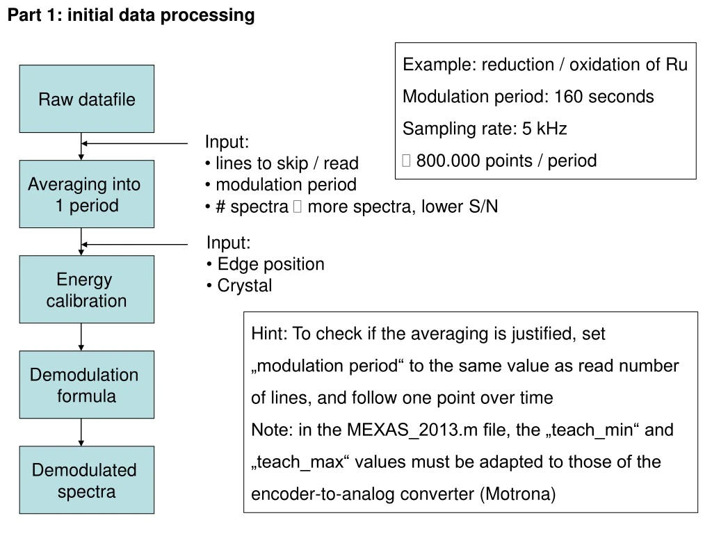
Part 1: initial data processing Example: reduction / oxidation of Ru Modulation period: 160 seconds Sampling rate: 5 kHz 800.000 points / period Raw datafile • Input: • lines to skip / read • modulation period • # spectra more spectra, lower S/N Averaging into 1 period • Input: • Edge position • Crystal Energy calibration Hint: To check if the averaging is justified, set „modulation period“ to the same value as read number of lines, and follow one point over time Note: in the MEXAS_2013.m file, the „teach_min“ and „teach_max“ values must be adapted to those of the encoder-to-analog converter (Motrona) Demodulation formula Demodulated spectra
Part 2: processing of demodulated spectra A: Quantative analysis of a simple square wave excitation / response: excitation response A(t)sin = π/4 (2n – 1) A(t)SW • Demodulated spectrum needs to be scaled accordingly • Easiest way is to scale the edge step • Edge-step(demod) = Edge-step(full) * 2 / π • To verify, compare to difference spectrum
Part 3: fitting of demodulated spectra Demodulated spectra Select phi for max. amplitude Scale correctly Fit EXAFS of full spec. Fit EXAFS of demod. spec. König et al, J. Phys. Chem. C (2012) doi: 10.1021/jp306022k
Part 2: processing of demodulated spectra B: Qualitative analysis of a not-so-simple excitation / response: Baurecht & Fringeli, Rev. Sci. Inst. 2001 In practice, phase-resolved modulation spectra are not only the basis for kinetic analysis but may be very useful for the separation of heavily overlapped absorption bands. A prerequisite, however, is that the two overlapping signals result from parts in the stimulated system that exhibit different kinetics, which is manifested by different phase lags with respect to the stimulation. Under this condition the maxima of the corresponding signals appear in different phase-resolved spectra, i.e., at different phase settings ΦPSD. Consequently, the amplitude zero crossings also occur in different spectra which are 90° apart from the corresponding spectra containing the maxima. This feature of PSD may be most efficient for the separation of a weak signal from an intense overlapping one. In this case, the operator controlled ΦPSD has to be selected in such a manner that the strong signal vanishes completely, thus enabling the experimental determination of the relevant parameters of the weak band, such as position, half width, and absorbance amplitude A.
Part 2: processing of demodulated spectra B: Qualitative analysis of a not-so-simple excitation / response: „raw“ demodulated spectra in k2 weighting Signal vs. phase angle at selected k Minority species can best be detected where major species go through zero König et al, J. Catal (2013) doi: 10.1016/j.jcat.2013.05.002
Part 3: fitting of demodulated spectra For quantitative analysis, you need to have a model Signal(total) = Signal (A1) + Signal (A2) Fourier(total) = Fourier (A1) + Fourier (A2) Demod (total) = Demod (A1) + Demod (A2) • Scaling factors for Demod (A1) and Demod (A2) • Fitting procedure is the same as before
Additional toys: • „MEXAS_demod_splitter.m“ - Split the file with demodulated spectra • „MEXAS_demod_phase_max.m“ - look at phase angles vs. k / amplitude vs. K • „MEXAS_theoretical2.m“ - process „synthetic“ spectra • „demod_theoretical_fourier_coefficients.xls“ – calculate Fourier coefficients for different functions