Download

1 / 21
210 likes | 421 Views
Detecting non-stationary in the unit hydrograph. Barry Croke 1,2 , Joseph Guillaume 2 , Mun-Ju Shin 1 1 Department of Mathematics 2 Fenner School for Environment and Society. Outline. Data analysis methods – detecting variability in the shape of the UH without resorting to a model

E N D
Detecting non-stationary in the unit hydrograph Barry Croke1,2, Joseph Guillaume2, Mun-Ju Shin1 1Department of Mathematics 2Fenner School for Environment and Society
Outline • Data analysis methods – detecting variability in the shape of the UH without resorting to a model • Adopting a UH model to explore variability in the UH shape between calibration periods • Comparison between different models • Testing structures of the non-linear module, and attempting to capture the variability in the UH shape
Data analysis methods • Direct estimation for Axe Creek • 49 peaks accepted in total • 13 large peaks (>4cumecs) • 28 small peaks (<3cumecs) Croke, 2006. A technique for deriving the average event unit hydrograph from streamflow-only data for quick-flow-dominant catchments, Advances in Water Resources. 29, 493-502, doi:10.1016/j.advwatres.2005.06.005.
Pareto analysis of cross-validation results • Identify one or more models per calibration period, and calculate performance in each calibration period • Ignore dominated models - inferior in all periods, retain the rest – no reason to eliminate them • Consider the range of non-dominated performance (RNDP) • Croke, 2010. Exploring changes in catchment response characteristics: Application of a generic filter for estimating the effective rainfall and unit hydrograph from an observed streamflowtimeseries, BHS2010. http://www.hydrology.org.uk/assets/2010%20papers/077Croke.pdf
Comparison of different models • IHACRES-CMD (Croke and Jakeman, 2004), 2 stores model used • fixed parameters: e=1 (potential evapotranspiration data used); d=200 • calibrated parameters: f=(0.5-1.3); tau_q=(0-10); tau_s=(10-1000); v_s=(0-1) • GR4J (Perrin, 2000, 2003), 4 parameters • SIMHYD (Chiew et al., 2002), 9 parameter version used (Podger, 2004) • Sacramento (Burnash et al., 1973), 13 parameters • Calibration algorithm: Shuffled Complex Evolution algorithm
Questions • What is the Range of Non-Dominated Performance (RNDP) across all periods? • What is the RNDP in each period? Is it low even though total RNDP is high? Why? • Which rainfall-runoff model has more Pareto-dominated models? • Which non-dominated model has the worst performance in each period? Is it consistently the same dataset (pattern)? Is there reason for that period to be problematic?
Results • Range of non-dominated performance (RNDP) is >0.1 for all catchments, but highly variable • 3 catchments (Allier, Ferson and Real) have periods that increase the RNDP with R2 (NSE) • RNDP reduced when R2log is used • GR4J has the most non-dominated cases • Worst models are SIMHYD (R2 ) and Sacremento (R2log ) • Five catchments (Durance, Ferson, Garonne, Kamp-zwettle and Real) have pattern of problematic behaviour (from the viewpoint of the models)
Exploring structure of non-linear module • Performance of stationary UH • Modified structure to permit variation based on catchment wetness • Compensating for suspected intense events
CMD module formulations • Stationary UH • Linear • Bilinear • Sin • Exponential • Power law • Variable UH • 2 effective rainfall time series • Intense events
Adopted structures • Most common: sinusoidal (9 catchments) • Mostly low order Nash cascades (2-3 stores)
Conclusion • A key source of non-stationarity in many catchments is variability in the shape of the UH • Seen as a trend in model residual against observed flow – not present in when plotted against modelled flow, so produced by an unknown driver • Hypothesis: variability is a result of event-to-event variations in rainfall intensity, and is predominantly a problem when using daily data • Need to overcome this before addressing smaller effects