Download
1 / 93
1.01k likes | 1.35k Views
Array and Matrix Operations. Dr. Marco A. Arocha INGE3016-MATLAB Sep 11, 2007, Dic 7, 2012. Array Operations. Array Addition. With 1D arrays : >> A=[1 3 5 ]; >> B=[2 4 6]; >> A+B ans = 3 7 11. With 2D arrays : >> A=[1 3 5; 2 4 6] A = 1 3 5

E N D
Array and Matrix Operations Dr. Marco A. Arocha INGE3016-MATLAB Sep 11, 2007, Dic 7, 2012
Array Addition With 1D arrays: >> A=[1 3 5 ]; >> B=[2 4 6]; >> A+B ans = 3 7 11 With 2D arrays: >> A=[1 3 5; 2 4 6] A = 1 3 5 2 4 6 >> B=[-5 6 10; 2 0 9] B = -5 6 10 2 0 9 >> A+B ans = -4 9 15 4 4 15
Array Multiplication >> A=[1,3,5;2,4,6] A = 1 3 5 2 4 6 >> B=[2,3,4;-1,-2,-3] B = 2 3 4 -1 -2 -3 >> A.*B ans = 2 9 20 -2 -8 -18 Arrays must be of the same size
Array Division >> A=[2,4,6] A = 2 4 6 >> B=[2,2,2] B = 2 2 2 >> A./B % num/den Right division ans = 1 2 3 >> A.\B % den\num Left division ans = 1.0000 0.5000 0.3333
Array Exponentiation >> A=[2,4,6] A = 2 4 6 >> B=[2,2,2] B = 2 2 2 >> B.^A ans = 4 16 64
Special Cases: array <operator> scalarscalar<operator> array >> A+2 ans = 3 4 5 >> A-1 ans = 0 1 2 If one of the arrays is a scalar the following are valid expressions. Given: >> A=[1 2 3]; >> A.*5 ans = 5 10 15 >> A./2 ans 0.5 1.0 1.5 Dot is optional in the above two examples
Special Cases:array <operator> scalarscalar<operator> array Given: a=[1 2 3] If one of the arrays is a scalar the following are valid expressions: >> a*2 ans = 2 4 6 >> a.*2 ans = 2 4 6 >> a/2 ans = 0.5000 1.0000 1.5000 >> a./2 ans = 0.5000 1.0000 1.5000
Special Cases >> A=[5] A = 5 >> B=[2,4,6] B = 2 4 6 >> A.*B ans = 10 20 30 Period is optional here
The basic data element in the MATLAB language is the array • Scalar • 1x1 array • Vectors: 1-D arrays • Column-vector: m x 1 array • Row-vector: 1 x n array • Multidimensional arrays • m x n arrays
MATRIX • Special case of an array: n, columns m, rows Rectangular array
Square Matrix Square matrix of order three • m=n Can reference individual elements Main diagonal: [2,5,3], i.e, Ai,jwhere i=j Z=3*A(2,3)
Self-dimensioning Upon initialization, MATLAB automatically allocates the correct amount of memory space for the array—no declaration needed, e.g., a=[1 2 3]; % creates a 1 x 3 array % without previously separate memory for storage
Self-dimensioning Upon appending one more element to an array, MATLAB automatically resizes the array to handle the new element >> a=[2 3 4] % a contains 3 elements a = 2 3 4 >> a(4)=6 % now a contains 4 elements a = 2 3 4 6 >> a(5)=7 % now a contains 5 elements a = 2 3 4 6 7
More on appending elements to an array: >> a=[1 2 3] a = 1 2 3 >> a=[a 4] a = 1 2 3 4 >> b =[a; a] b = 1 2 3 4 1 2 3 4 >> c=[a; 2*b] c = 1 2 3 4 2 4 6 8 2 4 6 8
Self-dimensioning is aMATLAB key feature This MATLAB key feature is different from most programming languages, where memory allocation and array sizing takes a considerable amount of programming effort Due to this feature alone MATLAB is years ahead, such high level languages as: C-language, FORTRAN, and Visual Basic for handling Matrix Operations
Deleting array elements >>A=[3 5 7] A = 3 5 7 >> A(2)=[ ] A = 3 7 >> B=[1 3 5; 2 4 6] B = 1 3 5 2 4 6 >> B(2,:)=[ ] B = 1 3 5 Deletes row-2, all column elements
Storage mechanism for arrays • Two common ways of storage mechanism, • depending on language: • One row at a time: row-major order (*) • 1 3 5 2 4 6 3 5 7 A = 1 3 5 2 4 6 3 5 7 Row-3 Row-2 Row-1 • One column at a time: column-major order • 2 3 3 4 5 5 6 7 • Last one is the MATLAB way of array storage col-3 col-1 col-2 (*) C Language uses row-major order
Accessing Individual Elements of an Array >> A=[1 3 5; 2 4 6; 3 5 7] A = 1 3 5 2 4 6 3 5 7 >> A(2,3) % row 2, column 3 ans = 6 Two indices is the usual way to access an element
Accessing elements of an Array by a single subscript >> A=[1 3 5; 2 4 6; 3 5 7] A = 1 3 5 2 4 6 3 5 7 In memory they are arranged as: 1 2 3 3 4 5 5 6 7 If wetry to accessthemwithonly one index, e.g.: >> A(1) ans = 1 >> A(4) ans = 3 >> A(8) ans = 6 Recall: column-major order in memory
Accessing Elements of an Array by a Single Subscript >> A=[1 3 5; 2 4 6; 3 5 7] A = 1 3 5 2 4 6 3 5 7 With one index & colon operator: >> A(1:2:9) ans = 1 3 4 5 7 The index goes from 1 up to 9 in increments of 2, therefore the indices referenced are: 1, 3, 5, 7, 9, and the referenced elements are: A(1), A(3), A(5), A(7),and A(9) In memory A(1)=1 A(4)=3 A(7)=5 A(2)=2 A(5)=4 A(8)=6 A(3)=3 A(6)=5 A(9)=7
Example Add one unit to each element in A: Given: A(1:1:3;1:1:3)=1 Answer-1: for ii=1:1:9 A(ii)=A(ii)+1; end
Example, continuation Answer-2: • A(1:1:9)=A(1:1:9)+1; Answer-3: • A=A(1:1:9)+1; • % one index Answer-4: • A=A.*2; Answer-5: • A=A+1;
Exercise With one index, Referencing is OK, Initializing is not. Initialize this Matrixwith one index: for k =1:1:25 if mod(k,6)==1 A(k)='F'; % ‘F’ elements are in indices: 1, 7, 13, 19, and 25 else A(k)='M'; end end % looks beautiful but doesn’t work at all, elements are not distributed as desired % We can make reference to the elements of a 2-D array with one index % however we can’t initialize a 2-D array with only one index.
Accessing Elements of an Array >> A=[1 3 5; 2 4 6; 3 5 7] A = 1 3 5 2 4 6 3 5 7 >> A(2,:) ans = 2 4 6 (2, :) meansrow 2, all columns A colon alone “ : “ means all the elements of that dimension
Accessing Elements of an Array >> A=[1 3 5; 2 4 6; 3 5 7] A = 1 3 5 2 4 6 3 5 7 >> A(2:3, 1:2) ans = 2 4 3 5 Means: rows from 2 to 3, and columns from 1 to 2, referenced indices are: (2,1) (2,2) (3,1) (3,2) row,column
Vectorization • The term “vectorization” is frequently associated with MATLAB. • Means to rewrite code so that, instead of using a loop iterating over each scalar-element in an array, one takes advantage of MATLAB’s vectorization capabilities and does everything in one go. • It is equivalent to change a Yaris for a Ferrari
Vectorization Operations executed one by one: x = [ 1, 2, 3, 4, 5, 6, 7, 8, 9, 10 ]; y = zeros(size(x)); % to speed code for k = 1:1:size(x) y(k) = x(k)^3; end Vectorized code: x = [ 1 :1:10 ]; y = x.^3;
Vectorization Operations executed one by one: x = [ 1, 2, 3, 4, 5, 6, 7, 8, 9, 10 ]; y = zeros(size(x)); for ii = 1:1:size(x) y(ii) = sin(x(ii)); end Vectorized code: x = [ 1 :1:10 ]; y = sin(x);
Vectorization Operations executed one by one: x = [ 1, 2, 3, 4, 5, 6, 7, 8, 9, 10 ]; y = zeros(size(x)); for ii = 1:1:size(x) y(ii) = sin(x(ii))/x(ii); end Vectorized code: x = [ 1 :1:10 ]; y = sin(x)./x;
Vectorization Operations executed one by one: % 10th Fibonacci number (n=10) f(1)=0; f(2)=1; for k = 3:1:n f(k) = f(k-1)+f(k-2); end WRONG Vectorization: % 10th Fibonacci number (n=10) f(1)=0; f(2)=1; k= [ 3 :1:n]; f(k) = f(k-1)+f(k-2); CAN’T
Vectorization Operations executed one by one: % Find factorial of 5: 5! x=[1:1:5]; p=1; for ii = 1:1:length(x) p=p*x(ii); end Wrong Vectorization: Why this code doesn’t work?: x=[1:1:5]; p(1)=1; ii=2:1:length(x); p(ii)=p(ii-1)*x(ii);
Vectorization-Exercise: Vectorizethe following loop: for ii=1:1:n+1 tn(ii)=(to(ii-1)+to(ii+1))/2; end Note: to, the old temperatures array has been initialized previously, i.e., all elements already exist in memory Answer: ii=[1:1:n+1]; tn(ii)=(to(ii-1)+to(ii+1))/2;
Matrix Operations Follows linear algebra rules
Vector Multiplication • Dot product (or inner product or scalar product) • Adding the product of each pair of respective elements in A and B • A must be a row vector • B must be a column vector • A and B must have same number of elements
Vector Multiplication >> A=[1,5,6] A = 1 5 6 >> B=[-2;-4;0] B = -2 -4 0 >> A*B ans = -22 1*(-2)+5*(-4)+6*0=-22 ~ No period before the asterisk * ~ The result is a scalar ~ Compare this with array multiplication
A*B A B Matrix Multiplication • Compute the dot products of each row in A with each column in B • Each result becomes a row in the resulting matrix No commutative: AB≠BA
Matrix Multiplication Math Syntax: AB MATLAB Syntax: A*B (NO DOT) >> A=[1 3 5; 2 4 6] A = 1 3 5 2 4 6 >> B=[-2 4; 3 8; 12 -2] B = -2 4 3 8 12 -2 >> A*B ans = 67 18 80 28 Sample calculation: The dot product of row one of A and column one of B: (1*-2)+(3*3)+(5*12)=67
Transpose Columns become rows
Transpose MATLAB: >> A=[1,2,3;4,5,6;7,8,9] A = 1 2 3 4 5 6 7 8 9 >> A' ans = 1 4 7 2 5 8 3 6 9
Determinant • Transformation of a square matrix that results in a scalar • Determinant of A: |A| or det A • If matrix has single entry: A=[3] det A = 3
Determinant Example with matrix of order 2: >> A=[2,3;6,4] A = 2 3 6 4 >> det(A) ans = -10 MATLAB instructions
Matrix Exponentiation • A must be square: A2=AA (matrix multiplication) A3=AAA MATLAB >> A=[1,2;3,4] A = 1 2 3 4 >> A^2 ans = 7 10 15 22 >> A^3 ans = 37 54 81 118
Operators Comparison Array Operations Matrix Operations * / ^ • .* • ./ • .^ • “+” and “-” • apply to both array and matrix operations and produce same results
Operators Comparison Array Operations Matrix Operations a=[1,2,3,4,5]; b=[5,4,3,2,1]; c=a*b a=[1,2,3,4,5]; b=[5,4,3,2,1]; c=a.*b • Find the results of the two statements above, discuss the results
Operators Comparison Array Operations Matrix Operations a=[1,2,3,4,5]; b=[5,4,3,2,1]’; c=a*b a=[1,2,3,4,5]; b=[5,4,3,2,1]’; c=a.*b • Find the results of the two statements above, discuss the results
Operator Precedence You can build expressions that use any combination of arithmetic, relational, and logical operators. Precedence levels determine the order in which MATLAB evaluates an expression. Within each precedence level, operators have equal precedence and are evaluated from left to right. The precedence rules for MATLAB operators are shown in this list, ordered from highest precedence level to lowest precedence level: • Parentheses () • Transpose (.'), power (.^), complex conjugate transpose ('), matrix power (^) • Unary plus (+), unary minus (-), logical negation (~) • Multiplication (.*), right division (./), left division (.\), matrix multiplication (*), matrix right division (/), matrix left division (\) • Addition (+), subtraction (-) • Colon operator (:) • Less than (<), less than or equal to (<=), greater than (>), greater than or equal to (>=), equal to (==), not equal to (~=) • Element-wise AND (&) • Element-wise OR (|) • Short-circuit AND (&&) • Short-circuit OR (||)