Some Recent Developments in Remote Sensing of Ice Sheets

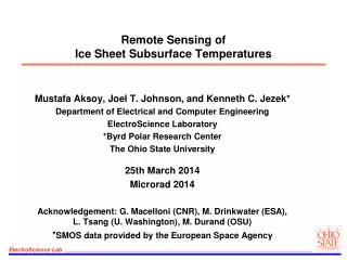
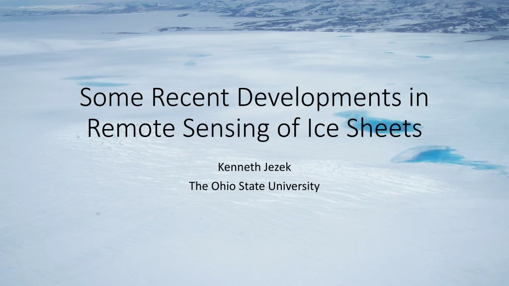
1. Some Recent Developments in Remote Sensing of Ice Sheets Kenneth Jezek The Ohio State University

2. Motivation • Limited capability to • capture 3-d detail of glacier bed and internal structure • determine ice sheet internal temperatures • Science Drivers • Internal temperature influences stiffness, which influences stress-strain relationship and therefore ice deformation and motion • Bed geometry is a strong control on ice flow • Research Goals • Measure ice sheet internal temperatures remotely (radiometry) • Image buried landscape as if the ice sheet were stripped away (radar) • Investigate advantages of combined active and passive measurements

3. Physics of the Problem

4. Principle of Tomographic Radar Sounding  air H Invert matrix to produce 3-d images of subsurface geometry D ice xi: received signal of sensor i; k: 4/; di: distance of sensor i; i: arrival angle; p: number of sensors; si: signal; q: number of signals; ni: noise; base • Received signals at each sensor:

5. Emission Physics 5 • In absence of scattering, thermal emission from ice sheet can be treated as a 0th order radiative transfer process • Similar to emission from the atmosphere: temperature profiling possible if strong variations in extinction with frequency (i.e. absorption line resonance) • Ice sheet has no absorption line but extinction does vary with frequency • Motivates investigating brightness temperatures as function of frequency

6. Progress in Radiometry SMAP, 2015

7. Evidence from SMOS SMOS data over Lake Vostok (East Antarctic Plateau) 25° 55° The analysis of SMOS data point out a relationship between Tb and Ice Thickness Brogioni, Macelloni, Montomoli, and Jezek, 2015

8. 500 MHz Model results suggest Tb sensitivity at depth and dependence on presence of subglacial water Modeled UHF Behavior for Antarctic Jezek and others, 2015

9. Greenland Brightness Temperatures Cloud Model, SMOS, SMAP • Cloud model Tb estimate based on temperature profiles derived from OIB thickness, CISM heat flux, RACMO SMB, MODIS surface temp. Parameter then corrected to match CC, NGRIP, GRIP temps. • 1.4 GHz data forced to align with SMOS data (black) using a constant multiplier. Same multiplier applied to other frequencies. • Variations are small at 1.4 GHz along flight path because temperature profiles are more uniform in depth. 500 MHz anomaly associated with region of assigned basal melt Frequency 0.5 GHz B Model 1.0 R “” 1.4 C “” 2.0 G “” SMOS Bla (thick) (Jan. 2014) SMAP B (thick) (April, 2015) Oswald and Gogineni, Subsurface Water Map

10. Antarctica-Greenland Brightness Temp vs. Frequency • Antarctic geophysical cases: low accumulation rates result in temp profiles that increase with depth • Strong changes in TB vs. frequency • Higher accumulation rates in Greenland (at least for GISP site) result in more uniform temp profile vs. depth • Smaller changes in TB vs. frequency • Need instrumentthat can capturethese variations Antarctica Blue: Simulated Profiles Red: GISP Data Blue: With Antenna Red: Without Antenna Greenland(GISP) Greenland(GISP)

11. Additional Factors Figure 7. Brightness temperature for changing the total thickness of the near surface low density layer. The discrete layer thickness is constant at 0.1 m. Variability is a consequence of recomputing the density function for each calculation. The red curve shows only the effect so the subsurface layers. The blue cure includes the loss at the air snow interface. Layering is important. At present, include statistical model of density with depth (Gaussian variability with a defined correlation length) Model layering effects using coherent and partially coherent radiative transfer models Working on interface roughness Yet to include layer conductivity at depth

12. Forward Model Assessment (Tan and others, 2015) Cloud DMRT/MEMLS Coherent • Used “Dome-C”-type physical parameters • Including density fluctuations with correlation length parameter • Results show: • Coherent effects can be significant if density correlation length << wavelength; otherwise good agreement between models

13. Greenland Retrieval Studies • Generated simulated 0.5-2 GHz observations of “GISP-like” ice sheets for varying physical properties (500 “truth” cases) • Including averaging over density fluctuations • For each truth case, generate 100 simulated retrievals with expected noise levels (i.e. ~ 1 K measurement noise per ~ 100 MHz bandwidth) • Select profile “closest” to simulated data as the retrieved profile, and examine temperature retrieval error • Errors in this simulation meet science requirements • Additional simulations continuing over Greenland flight path

14. OSU Ulta-WideBand Software Controlled Radiometer Presently building an instrument that can measure: • Ice sheet temperature at 10 m depth, 1 K accuracy • 10 m temperatures approximate the mean annual temperature, an important climate parameter • Depth-averaged temperature from 200 m to 4 km (max) ice sheet thickness, 1 K accuracy • Spatial variations in average temperature can be used as a proxy for improving temperature dependent ice-flow models • Temperature profile at 100 m depth intervals, 1 K accuracy • Remote sensing measurements of temperature-depth profiles can substantially improve ice flow models • Measurements all at minimum 10 km resolution • Time stamped and geolocated by latitude and longitude

15. Progress in Radar Tomography

16. Multi-frequency Images of Ice Sheet Surface Lake Crevasse Band Ice stream July 20, 2008, 17 km wide, 150 MHz radar tomography GISMO image (geocoded) of the upper surface of the ice sheet across Jacobshavn Glacier (right). 2000 Radarsat C-band image (center). Inset map from Radarsat mosaic (left). July 15, 2008, MERIS optical image (lower left). GISMO image located at about 69.3N, 48.3 W

17. Surface Elevation Validation Wu and others, 2011

18. Validation: basal topography accuracy Image: Ice thickness map of Jacobshavn, Greenland (2008) mosaiced from 2 GISMO swaths. Gray-scale indicates thickness. The lines locate Kansas University’s nadir ice sounder 2006 tracks. Graphs: Ice thickness inter-comparisons have 18m and 14m rms errors. 22 km 4.5 km

19. GISMO Basal Imagery Oblique downstream views of basal topography beneath the Greenland Ice Sheet compared with part of the now-exposed bed of the former Laurentide Ice Sheet near Norman Wells, Northwest Territories, Arctic Canada (60.3 N, 126.7 W; image ca 0.5 km in width). 5x20 Km 3-d image of the base of the ice sheet. Scene is an orthorectified mosaic located just south of the main Jacobshavn Drainage Channel Jezek and others, 2011

20. Basal Imaging: Southern Flank of Jacobshavn Glacier, Greenland Radarsat-1 image showing the location of the study area (red box) located about 14 km south of the main Jacobshavn Glacier drainage channel. Ice thickness in meters. Surface velocity vectors from radar interferometry. basal topography contours in m above the ellipsoid. Red (bright) and blue (weak) tones represent radar reflectivity. 5x20 km hill-shaded basal topography. Ice flow lines (red) are determined from Driving stress in PascalsColor tones correspond to radar reflectivity. Jezek and others, 2011

21. Radar Sounding of Russel Glacier: Nadir Tracking and Tomography Hill-shaded model of the tomography-derived basal topography (dark blue) overlaid on a hill-shaded model of the interpolated nadir-data topography (gray). In turn, these are overlaid on a lidar derived model of the ice-sheet, exposed-rock surface (light blue). Basal Topography estimate of IsunguataSermia Glacier computed by tomography (upper) and by interpolating nadir (lower). Driving stress overlaid on Landsat-7 image. Lakes (white patches) generally correspond to locations of low driving stress. Jezek, Wu, Paden, Leuschen, 2012

22. Example of shallow pockets at Umanaq, Greenland - 2011 IceBridge data

23. Example of shallow pockets at Umanaq: Intensity (top) and bed thickness (bottom) depth (3 km in air) 1160m Along track (20 km) cross track ground range (3km) 50 m Courtesy Wu, 2014

24. Anomalous Subsurface Object Approximate Location of the feature

25. Details on Subsurface Structure Intensity image Location of the data frame depth (3 km in air) Along track (3.75 km) Ice thickness cross track ground range (3 km) Ice thickness map in Polar stereo-graphic projection 100 m 530 m Courtesy Wu, 2014

26. Instrumentation Specifications Hybrid couplers

27. GISMO Radar Parameters and Configuration

28. Ultra-wideband software defined radiometer (UWBRAD) Diameter: 1.1 inches Cone Angle= 13.2° H = 37” 56 Turns Diameter: 10 inches UWBRAD=a radiometer operating 0.5 – 2 GHz for internal ice sheet temperature sensing Requires operating in unprotected bands, so interference a major concern Address by sampling entire bandwidth ( in 100 MHz channels) and implement real-time detection/mitigation/use of unoccupied spectrum Supported under NASA 2013 Instrument Incubator Program

29. Next Step: Radar and Radiometry • Difficult to model fine scale structure necessary to accurately correct Tb data for near surface scattering • Wideband radar may be suitable for characterizing scattering magnitudes • Peake’s equation relates emissivity to backscatter coefficient based on conservation of incoming, scattered and emitted power • Spaceborne systems already operate L-band radars and radiometers (Aquarius, SMAP) • Potential for integrating UWBRAD with wideband radars developed by CReSIS. Will require additional development of tomographic and bistatic-SAR techniques. 2016 experiment will underflyCReSIS data.

30. Antarctic and Greenland Field Deployments • IFAC will deploy an L-band radiometer at DOME-C November 2015-January 2016 (30-45 day campaign) • Plan to include UWBRAD tower deployment at DOME-C as part of the IFAC Project • Would be desirable to include full 13 channel system, but a 4 channel system could provide valuable information • Developing plan to deploy UWBRAD 4 channel system at DOME-C UWBRAD Enclosure • April or October 2016 Greenland Airborne Campaign • Continued discussions with Ken Borek Air, Ltd. for use of Bassler aircraft • Budget for 5 days/ 40 flight hours consistent with project plan Antenna

31. Summary • Radar Tomography: • Technique proven in limited instances • Provides necessary measurement of 3-d ice sheet internal structure and basal geometry • Requires more research to improve swath width and continuous coverage • Requires algorithm development for routine products useful for models • Wideband Radiometry • Operational L-band systems suggest brightness temperatures are sensitive to depth • Wideband simulations demonstrate that, within assumptions, physical temperature can be measured at depth • UWBRAD will be tested in October 2015 and April 2016 • Radar and Radiometry • Active and passive measurements may be required to correct radiometric data for scattering from the complex, near surface layers of the ice sheet