Exploring Graph Theory: Fundamentals and Applications

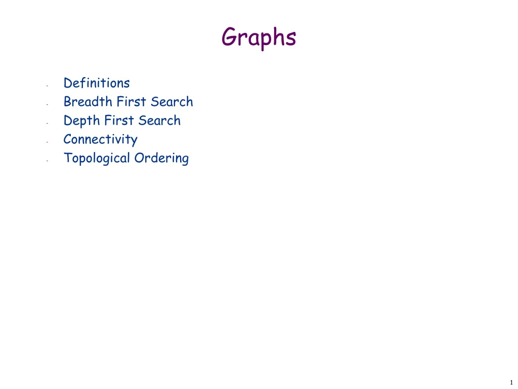
1. Graphs • Definitions • Breadth First Search • Depth First Search • Connectivity • Topological Ordering

2. 3.1 Basic Definitions and Applications

3. Undirected Graphs • Undirected graph. G = (V, E) • V = nodes. • E = edges between pairs of nodes. • Captures pairwise relationship between objects. • Graph size parameters: n = |V|, m = |E|. V = { 1, 2, 3, 4, 5, 6, 7, 8 } E = { 1-2, 1-3, 2-3, 2-4, 2-5, 3-5, 3-7, 3-8, 4-5, 5-6 }n = 8 m = 11

4. Some Graph Applications Graph Nodes Edges transportation street intersections highways communication computers fiber optic cables World Wide Web web pages hyperlinks social people relationships food web species predator-prey software systems functions function calls scheduling tasks precedence constraints circuits gates wires

5. World Wide Web • Web graph. • Node: web page. • Edge: hyperlink from one page to another. cnn.com netscape.com novell.com cnnsi.com timewarner.com hbo.com sorpranos.com

6. Ecological Food Web • Food web graph. • Node = species. • Edge = from prey to predator. Reference: http://www.twingroves.district96.k12.il.us/Wetlands/Salamander/SalGraphics/salfoodweb.giff

7. Graph Representation: Adjacency Matrix • Adjacency matrix. n-by-n matrix with Auv = 1 if (u, v) is an edge. • Two representations of each edge. • Space proportional to n2. • Checking if (u, v) is an edge takes (1) time. • Identifying all edges takes (n2) time. 1 2 3 4 5 6 7 8 1 0 1 1 0 0 0 0 0 2 1 0 1 1 1 0 0 0 3 1 1 0 0 1 0 1 1 4 0 1 0 1 1 0 0 0 5 0 1 1 1 0 1 0 0 6 0 0 0 0 1 0 0 0 7 0 0 1 0 0 0 0 1 8 0 0 1 0 0 0 1 0

8. Graph Representation: Adjacency List • Adjacency list. Node indexed array of lists. • Two representations of each edge. • Space proportional to m + n. • Checking if (u, v) is an edge takes O(deg(u)) time. • Identifying all edges takes (m + n) time. degree = number of neighbors of u 1 2 3 1 3 4 5 2 8 7 1 2 5 3 4 2 5 2 3 4 6 5 5 6 7 3 8 8 3 7

9. Paths and Connectivity • Def. A path in an undirected graph G = (V, E) is a sequence P of nodes v1, v2, …, vk-1, vk with the property that each consecutive pair vi, vi+1 is joined by an edge in E. • Def. A path is simple if all nodes are distinct. • Def. An undirected graph is connected if for every pair of nodes u and v, there is a path between u and v.

10. Cycles • Def. A cycle is a path v1, v2, …, vk-1, vk in which v1 = vk, k > 2, and the first k-1 nodes are all distinct. cycle C = 1-2-4-5-3-1

11. Trees • Def. An undirected graph is a tree if it is connected and does not contain a cycle. • Theorem. Let G be an undirected graph on n nodes. Any two of the following statements imply the third. • G is connected. • G does not contain a cycle. • G has n-1 edges.

12. Rooted Trees • Rooted tree. Given a tree T, choose a root node r and orient each edge away from r. • Importance. Models hierarchical structure. root r parent of v v child of v a tree the same tree, rooted at 1

13. Phylogeny Trees • Phylogeny trees. Describe evolutionary history of species.

14. GUI Containment Hierarchy • GUI containment hierarchy. Describe organization of GUI widgets. Reference: http://java.sun.com/docs/books/tutorial/uiswing/overview/anatomy.html

15. 3.2 Graph Traversal

16. Connectivity • s-t connectivity problem. Given two node s and t, is there a path between s and t? • s-t shortest path problem. Given two node s and t, what is the length of the shortest path between s and t? • Applications. • Friendster. • Maze traversal. • Kevin Bacon number. • Fewest number of hops in a communication network.

17. L1 L2 s L n-1 Breadth First Search • BFS intuition. Explore outward from s in all possible directions, adding nodes one "layer" at a time. • BFS algorithm. • L0 = { s }. • L1 = all neighbors of L0. • L2 = all nodes that do not belong to L0 or L1, and that have an edge to a node in L1. • Li+1 = all nodes that do not belong to an earlier layer, and that have an edge to a node in Li. • Theorem. For each i, Li consists of all nodes at distance exactly ifrom s. There is a path from s to t iff t appears in some layer.

18. Breadth First Search Algorithm

19. Breadth-First Search - Idea • Given a graph G = (V, E), start at the source vertex “s” and discover which vertices are reachable from s • At any time there is a “frontier” of vertices that have been discovered, but not yet processed • Next pick the nodes in the frontier in sequence and discover their neighbors, forming a new “frontier” • Breadth-first search is so named because it visits vertices across the entire breadth of this frontier before moving on 2 1 2 2 s s s 1 2 2 1 2

20. BFS - Continued • Represent the final result as follows: • For each vertex v e V, we will store d[v] which is the distance (length of shortest path) from s to v • Distance between a vertex “v” and “s” is defined to be the minimum number of edges on a path from “s” to “v” • Note that d[s] = 0 • We will also store a predecessor (or parent) pointer pred[v] or p[v], which indicates the first vertex along the shortest path if we walk from v backwards to s • We will let prev[s] or p[s] = 0 • Notice that these predecessor pointers are sufficient to reconstruct the shortest path to any vertex

21. BFS – Implementation • Initially all vertices (except the source) is colored white, meaning they have not been discovered just yet • When a vertex is first discovered, it is colored gray (and is part of the frontier) • When a gray vertex is processed, it becomes black 2 1 2 2 s s s 1 2 2 1 2

22. BFS - Implementation • The search makes use of a FIFO queue, Q • We also maintain arrays • color[u], which holds the color of vertex u • either white, gray, black • pred[u], which points to the predecessor of u • The vertex that discovered u • d[u], the distance from s to u 2 1 2 2 s s s 1 2 2 1 2

23. BFS –Another way of Implemenattion • BFS(G, s){ • for each u in V- {s} { // Initialization • color[u] = white; • d[u] = INFINITY; • pred[u] = NULL; • } //end-for • color[s] = GRAY; // initialize source s • d[s] = 0; • pred[s] = NULL; • Q = {s}; // Put s in the queue • while (Q is nonempty){ • u = Dequeue(Q); // u is the next vertex to visit • for each v in Adj[u] { • if (color[v] == white){ // if neighbor v undiscovered • color[v] = gray; // … mark is discovered • d[v] = d[u] + 1; // … set its distance • pred[v] = u; // … set its predecessor • Enqueue(v); //… put it in the queue • } //end-if • } //end-for • color[u] = black; // we are done with u • } //end-while • } //end-BFS

24. BFS - Analysis • Let n = |V| and e = |E| • Observe that the initial portion requires q(n) • The real meat is through the traversal loop • Since we never visit a vertex twice, the number of times we go through the loop os at most n (exactly n assuming each vertex is reachable from the source) • The number of iterations through the inner loop is proportional to deg(u) • Summing up over all vertices we have • T(n) = n + Sum_{v e V} deg[v] = n + 2e = q(n+e)

25. Breadth First Search • Property. Let T be a BFS tree of G = (V, E), and let (x, y) be an edge of G. Then the level of x and y differ by at most 1. L0 L1 L2 L3

26. Breadth First Search: Analysis • Theorem. The above implementation of BFS runs in O(m + n) time if the graph is given by its adjacency representation. • Pf. • Easy to prove O(n2) running time: • at most n lists L[i] • each node occurs on at most one list; for loop runs  n times • when we consider node u, there are  n incident edges (u, v),and we spend O(1) processing each edge • Actually runs in O(m + n) time: • when we consider node u, there are deg(u) incident edges (u, v) • total time processing edges is uV deg(u) = 2m ▪ each edge (u, v) is counted exactly twicein sum: once in deg(u) and once in deg(v)

28. Depth First Search : The Concept • Consider searching the way out from a maze. • As you enter a location of the maze, paint some graffiti on the wall to remind yourself that you were there • Successively travel from room to room as long as you come to a place you have not already been • When you return to the same room, try a different door (assuming it goes somewhere you have not been before) • When all doors have been tried in a room, backtrack • Same idea in trying to find a door out of a puzzle

29. DFS Algorithm Recursive Version 1

31. DFS Stack Version 2

32. DFS – Version 3 (CLR Book) • Assume you are given a digraph G = (V, E) • The same algorithm works for undirected graphs but the resulting structure imposed on the graph is different • We use 4 auxiliary arrays • color[u] • White – undiscovered • Gray – discovered but not yet processed • Black – finished processing • pred[u], which points to the predecessor of u • The vertex that discovered u • 2 timestamps: Purpose will be explained later • d[u]: Time at which the vertex was discovered • Not to be confused with distance of u in BFS! • f[u]: Time at which the processing of the vertex was finished

33. DFS – Version 3 • DFS(G, s){ • for each u in V { // Initialization • color[u] = white; • pred[u] = NULL; • } //end-for • time = 0; • for each u in V • if (color[u] == white) // Found an undiscovered vertex • DFSVisit(u); // Start a new search there • } // end-DFS • DFSVisit(u){ // Start a new search at u • color[u] = gray; // Mark u visited • d[u] = ++time; • for each v in Adj[u] { • if (color[v] == white){ // if neighbor v undiscovered • pred[v] = u; // … set its predecessor • DFSVisit(v); // …visit v • } //end-if • } //end-for • color[u] = black; // we are done with u • f[u] = ++time; • } //end-while • } //end-DFSVisit

34. DFS - Example d • DFS imposes a tree structure (actually a collection of trees or a forest) on the structure of the graph • This is just the recursion tree, where the edge (u, v) arises when processing vertex “u” we call DFSVisit(v) for some neighbor v a e d 11/14 C 1/10 f b a f b C 2/5 6/9 e 12/13 F B c g 3/4 c 7/8 g C

35. Connected Component • Connected component. Find all nodes reachable from s. • Connected component containing node 1 = { 1, 2, 3, 4, 5, 6, 7, 8 }.

36. Flood Fill • Flood fill. Given lime green pixel in an image, change color of entire blob of neighboring lime pixels to blue. • Node: pixel. • Edge: two neighboring lime pixels. • Blob: connected component of lime pixels. recolor lime green blob to blue

37. Flood Fill • Flood fill. Given lime green pixel in an image, change color of entire blob of neighboring lime pixels to blue. • Node: pixel. • Edge: two neighboring lime pixels. • Blob: connected component of lime pixels. recolor lime green blob to blue

38. Connected Component • Connected component. Find all nodes reachable from s. • Theorem. Upon termination, R is the connected component containing s. • BFS = explore in order of distance from s. • DFS = explore in a different way. R s u v it's safe to add v

39. 3.4 Testing Bipartiteness

40. Bipartite Graphs • Def. An undirected graph G = (V, E) is bipartite if the nodes can be colored red or blue such that every edge has one red and one blue end. • Applications. • Stable marriage: men = red, women = blue. • Scheduling: machines = red, jobs = blue. a bipartite graph

41. Testing Bipartiteness • Testing bipartiteness. Given a graph G, is it bipartite? • Many graph problems become: • easier if the underlying graph is bipartite (matching) • tractable if the underlying graph is bipartite (independent set) • Before attempting to design an algorithm, we need to understand structure of bipartite graphs. v2 v2 v3 v1 v4 v3 v5 v6 v4 v5 v6 v7 v1 v7 a bipartite graph G another drawing of G

42. An Obstruction to Bipartiteness • Lemma. If a graph G is bipartite, it cannot contain an odd length cycle. • Pf. Not possible to 2-color the odd cycle, let alone G. bipartite(2-colorable) not bipartite(not 2-colorable)

43. Bipartite Graphs • Lemma. Let G be a connected graph, and let L0, …, Lk be the layers produced by BFS starting at node s. Exactly one of the following holds. (i) No edge of G joins two nodes of the same layer, and G is bipartite. (ii) An edge of G joins two nodes of the same layer, and G contains an odd-length cycle (and hence is not bipartite). L2 L3 L1 L2 L3 L1 Case (ii) Case (i)

44. Bipartite Graphs • Lemma. Let G be a connected graph, and let L0, …, Lk be the layers produced by BFS starting at node s. Exactly one of the following holds. (i) No edge of G joins two nodes of the same layer, and G is bipartite. (ii) An edge of G joins two nodes of the same layer, and G contains an odd-length cycle (and hence is not bipartite). • Pf. (i) • Suppose no edge joins two nodes in the same layer. • By previous lemma, this implies all edges join nodes on same level. • Bipartition: red = nodes on odd levels, blue = nodes on even levels. L2 L3 L1 Case (i)

45. Bipartite Graphs • Lemma. Let G be a connected graph, and let L0, …, Lk be the layers produced by BFS starting at node s. Exactly one of the following holds. (i) No edge of G joins two nodes of the same layer, and G is bipartite. (ii) An edge of G joins two nodes of the same layer, and G contains an odd-length cycle (and hence is not bipartite). • Pf. (ii) • Suppose (x, y) is an edge with x, y in same level Lj. • Let z = lca(x, y) = lowest common ancestor. • Let Li be level containing z. • Consider cycle that takes edge from x to y,then path from y to z, then path from z to x. • Its length is 1 + (j-i) + (j-i), which is odd. ▪ z = lca(x, y) (x, y) path fromy to z path fromz to x

46. Obstruction to Bipartiteness • Corollary. A graph G is bipartite iff it contain no odd length cycle. 5-cycle C bipartite(2-colorable) not bipartite(not 2-colorable)

47. 3.5 Connectivity in Directed Graphs

48. Directed Graphs • Directed graph. G = (V, E) • Edge (u, v) goes from node u to node v. • Ex. Web graph - hyperlink points from one web page to another. • Directedness of graph is crucial. • Modern web search engines exploit hyperlink structure to rank web pages by importance.

49. Graph Search • Directed reachability. Given a node s, find all nodes reachable from s. • Directed s-t shortest path problem. Given two node s and t, what is the length of the shortest path between s and t? • Graph search. BFS extends naturally to directed graphs. • Web crawler. Start from web page s. Find all web pages linked from s, either directly or indirectly.

50. Strong Connectivity • Def. Node u and v are mutually reachable if there is a path from u to v and also a path from v to u. • Def. A graph is strongly connected if every pair of nodes is mutually reachable. • Lemma. Let s be any node. G is strongly connected iff every node is reachable from s, and s is reachable from every node. • Pf.  Follows from definition. • Pf.  Path from u to v: concatenate u-s path with s-v path. Path from v to u: concatenate v-s path with s-u path. ▪ ok if paths overlap s u v