Download
1 / 93
960 likes | 1.03k Views
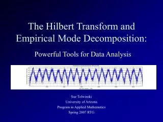
Learn about the Empirical Mode Decomposition method for data analysis, including the need for decomposition, Hilbert Transform, intrinsic mode functions, and the process of sifting to extract IMF components. Understand the significance of adaptive methods and sparse representation in analyzing nonstationary and nonlinear data.

E N D
Goal of Data Analysis • To define time scale or frequency. • To define energy density. • To define joint frequency-energy distribution as a function of time. • To do this, we need a AM-FM decomposition of the signal: X(t) = A(t) cosθ(t), where A(t) defines local energy and θ(t) defines the local frequency. This is a Generalized Fourier Expansion.
Need for Decomposition • Hilbert Transform (and all other IF computation methods) offers meaningful Instantaneous Frequency for IMFs. • For complicate data, there should be more than one independent component at any given time. • The decomposition should be adaptive in order to study data from nonstationary and nonlinear processes. • Frequency space operations are difficult to track temporal changes.
Why Hilbert Transform is not enough? Even though mathematicians told us that the Hilbert transform exists for all functions of Lp-class.
Problems on ‘Envelope’ A seemingly simple proposition but it is not so easy.
Observations • None of the two “envelopes” seem to make sense in term of Generalized Fourier Expansion (GFE): • The Hilbert transformed amplitude oscillates too much. • The line connecting the local maximum is almost the tracing of the data. • It turns out that, though Hilbert transform exists, the simple Hilbert transform does not make sense physically. • For “envelopes” to make sense in terms of GFE, the necessary condition for Hilbert transformed amplitude to make sense is for IMF.
Observations • For each IMF, the envelope in GFE will make sense. • For complicate data, we have to decompose it before attempting envelope construction. • To be able to determine the envelope is equivalent to AM & FM decomposition.
Observations • Even for this well behaved function, the amplitude from Hilbert transform does not serve as an “envelope” well. One of the reasons is that the function has two spectrum lines. • Hilbert Transform represents higher frequency better. • Complications for more complex functions are many. • Here, the empirical envelope seems reasonable.
Empirical Mode Decomposition • Mathematically, there are infinite number of ways to decompose a functions into a complete set of components. • The ones that give us more physical insight are more significant. • In general, the fewer the number of representing components, the higher the information content: Sparse representation. • The adaptive method will represent the characteristics of the signal better. • EMD is an adaptive method that can generate infinite many sets of IMF components to represent the original data.
Empirical Mode DecompositionSifting : to get one IMF component
Empirical Mode DecompositionSifting : to get one IMF component
Empirical Mode DecompositionSifting : to get all the IMF components
Empirical Mode DecompositionSifting : to get all the IMF components
Empirical Mode DecompositionSifting : to get all the IMF components
Empirical Mode DecompositionSifting : to get all the IMF components
Observations • All IMF components are the sums of spline functions. • We selected cubic natural spline tomaintain the maximum smoothness. • We will discuss spline function next time.
The Effects of Sifting • The first effect of sifting is to eliminate the riding waves : to make the number of extrema equals to that of zero-crossing. • The second effect of sifting is to make the envelopes symmetric. The consequence is to make the amplitudes of the oscillations more even.
Critical Parameters for EMD • The maximum number of sifting allowed to extract an IMF, N. • The criterion for accepting a sifting component as an IMF, the Stoppage criterion S. • Therefore, the nomenclature for the IMF are CE(N, S) : for extrema sifting CC(N, S) : for curvature sifting
The Stoppage Criteria : S and SD A. The S number : S is defined as the consecutive number of siftings, in which the numbers of zero-crossing and extrema are the same for these S siftings. B. If the mean is smaller than a pre-assigned value. C. Fixed sifting (iterating) time. D. SD is small than a pre-set value, where
Curvature Sifting Hidden Scales