Raytracing method application to the wavefiled decomposition

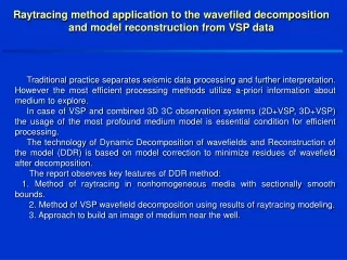
1. Raytracing method application to the wavefiled decomposition and model reconstruction from VSP data Traditional practice separates seismic data processing and further interpretation. However the most efficient processing methods utilize a-priori information about medium to explore. In case of VSP and combined 3D 3C observation systems (2D+VSP, 3D+VSP) the usage of the most profound medium model is essential condition for efficient processing. The technology of Dynamic Decomposition of wavefields and Reconstruction of the model (DDR) is based on model correction to minimize residues of wavefield after decomposition. The report observes key features of DDR method: 1. Method of raytracing in nonhomogeneous media with sectionally smooth bounds. 2. Method of VSP wavefield decomposition using results of raytracing modeling. 3. Approach to build an image of medium near the well.

2. Medium model definition Geometry of the model is defined as a set of points laying on sectionally smooth bounds. For next calculations smooth bounds are approximated by parametric cubic splines which allows to describe ambiguous bounds. The criteria of approximation is a curvature restriction. The bound is defined as a set of points on the spline between special end points – break points or another bound intersection. Maximum deviation of the chord between two consequent points from the spline is limited by preset value. Physical parameters of the model are defined on the bounds. The pressure, shear wave velocity and density are interpolated between bounds producing gradients.

3. Observation system For a case study the observation system with non-straight well and two shot points was defined. Distance between receivers in the well is 20 meters. Both shot points are located with offset 2500 meters.

4. - origin point of the i-th chord - pressure wave velocity - absolute value of velocity gradient - direction of the tangent to ray trajectory - direction of the velocity gradient Raytracing in gradient medium with sectionally smooth bounds The method of raytracing from arbitrary point in arbitrary direction was developed for the considered model. In general velocity gradient is not a constant so raytracing is performed step by step. Direction and length of a step is set according to parameters of the medium in origin point. The step defines chord Hi of a circle which is a true ray trajectory. The first step is made along the chord which has F angle to the ray direction. The F value is a parameter of the method and it defines accuracy of a solution. The less F value is the better the chord fits the circle. A chord value are calculated by given formula: , where: (i=0,1,….N)

5. Refraction-reflection effects are considered at a chord intersection with a bound by the following algorithm: A tangent to the bound in intersection point is drawn. Then the tangential component of refraction vector of incoming ray with defined type is calculated. This component is used for calculation of orthogonal component of refraction vector of outgoing reflected or refracted (converted or non-converted) ray. Refraction vector of incoming ray of wave type and vector of tangent to the bound in intersection point and orthogonal vector of the bound. Lets separate refraction vector of incoming ray to the orthogonal and tangential components: From the law of tangential component invariance: it’s easy to represent orthogonal component of refraction vector of the reflected/refracted ray: Thus we have complete vector of wave refraction (and the ray direction) just after bound instersection.

6. Calculation of model wave fields Model wave field was calculated by the method of finite differences on the grid with 2m step. The source was calculated analytically in the 100m radius. High-frequency noise on the grid was no more than 10% in the frequency range 0 - 62.5 – 125Hz. Inverse wave scattering on model boundaries was no more then 0.5%. X component of calculated field Z component of calculated field

7. Calculation of the wave parameters To calculate parameters of the wave with given type, it’s necessary to determine the source angle of the ray which hits exact receiver. In case of all such rays are found it’s possible to calculate travelling time, amplitude and polarization of the wave in the receiver. Thus the method allows to obtain amplitudes, polarization parameters and arrival times for every type of the wave. Example of reflected wave raytracing

8. Hodographs of the non-converted and converted reflected waves, calculated by the ray method

9. To illustrate accuracy of polarization parameters calculation, initial XYZ field was rotated to the polarization of converted transferred PS wave from the first bound: R componentP component

10. Amplitudes of the direct wave calculated by the ray-tracing (red) and finite difference (green) methods.

11. Wave detection and subtraction When hodograph and polarization parameters of the wave are known, it’s possible to subtract it from initial wave field without influence of the interference effects. Thus, by the sequential wave subtraction in the order of amplitudes decreasing, it’s possible to reach full wave field analysis up to multiple reflection/refraction ray paths. Hodograph of the converted wave

12. Wavefield after subtraction of a converted wave Subtracted wave

13. Definition of the a-priori model Model correctionby thefirst breaks times Bound selection Calculate the parameters of the waves, scattered by the selected bound Definition and subtraction of the scattered waves Imaging from subtracted waves of different types Test for the model and the image agreement Model correction DDR method If all boundaries are corrected Exit • Results: • -model of the medium • detected waves of all types • - image of the medium from waves of all types

14. DDR interface conception Wave field with hodograph Model and rays

15. Results • New algorithms and programs for fast ray tracing in complicated medium was developed. • Ray-tracing method is proved by comparison with finite difference of the modeling results. • Demonstrated elements of the combined system of data processing and interpretation, called Dynamic wave fields Decomposition with model Reconstruction. Greetings The authors express their gratitude to SEPTAR company for the model which was used for comparison of finite difference and ray-tracing method.