Download
1 / 42
430 likes | 500 Views
This lecture covers various network models such as Erdos–Renyi random graphs, small-world networks, scale-free networks, and hierarchical models. Learn about degree distributions, clustering coefficients, average diameters, and the stubs method in constructing generalized random graphs. Discover the characteristics and construction methods of different network models.

E N D
Network (graph) Models Lecture 6
Network models We will cover the following network models: • Erdos–Renyi random graphs • Generalized random graphs (with the same degree distribution as the data networks) • Small-world networks • Scale-free networks • Hierarchical model • Geometric random graphs
Erdos–Renyi random graphs (ER) • Model a data network G(V,E) with |V|=n and |E|=m • An ER graph that models G is constructed as follows: • It has n nodes • Edges are added between pairs of nodes uniformly at random with the same probability p • Two (equivalent) methods for constructing ER graphs: • Gn,p: pick p so that the resulting model network has m edges • Gn,m: pick randomly m pairs of nodes and add edges between them with probability 1
Erdos–Renyi random graphs (ER) • Number of edges, |E|=m, in Gn,pis: • Average degree is:
Erdos–Renyi random graphs (ER) • Many properties of ER can be proven theoretically (See: Bollobas, "Random Graphs," 2002) • Example: • When m=n/2,suddenly the giant component emerges, i.e.: • One connected component of the network has O(n) nodes • The next largest connected component has O(log(n)) nodes
Probability of drawing a graph of m edges • Look familiar? • The mean value of m • The mean degree of graph is
DEGREE DISTRIBUTION OF A RANDOM GRAPH probability of missing N-1-k edges Select k nodes from N-1 probability of having k edges As the network size increases, the distribution becomes increasingly narrow—we are increasingly confident that the degree of a node is in the vicinity of <k>. Network Science: Random Graphs
DEGREE DISTRIBUTION OF A RANDOM GRAPH For largeNand small k, we can use the following approximations: for Network Science: Random Graphs
POISSON DEGREE DISTRIBUTION For largeNand small k, we arrive to the Poisson distribution: Network Science: Random Graphs
Erdos–Renyi random graphs (ER) • The degree distribution is binomial: • For large n, this can be approximated with Poisson distribution: where z is the average degree • However, many real world networkshave power-law degree distribution
Erdos–Renyi random graphs (ER) • Clustering coefficient, C, of ER is low (for low p) • C=p, since probability p of connecting any two nodes in an ER graph is the same, regardless of whether the nodes are neighbors • However, many real world networkshave high clustering coefficients
Erdos–Renyi random graphs (ER) • Average diameter of ER graphs is small • It is equal to • Real networks alsohave small average diameters • Summary
Generalized random graphs (ER-DD) • Preserve the degree distribution of data (“ER-DD”) • Constructed as follows: • An ER-DD network has n nodes (so does the data) • Edges are added between pairs of nodes using the “stubs method” [configuration model discussed earlier]
Generalized random graphs (ER-DD) • The “stubs method” for constructing ER-DD graphs: • The number of “stubs” (to be filled by edges) is assigned to each node in the model network according to the degree distribution of the real network to be modeled • Edges are created between pairs of nodes with “available” stubs picked at random • After an edge is created, the number of stubs left available at the corresponding “end nodes” of the edges is decreased by one • Multiple edges between the same pair of nodes are not allowed
Generalized random graphs (ER-DD) • Summary • 2 global network properties are matched by ER-DD
Small-world networks (SW) • Watts and Strogatz, 1998 • Created from regular ring lattices by random rewiring of a small percentage of their edges • E.g.
Small-world networks (SW) • SW networks have: • High clustering coefficients – introduced by “ring regularity” • Large average diameters of regular lattices – fixed by randomly re-wiring a small percentage of edges • Summary
Scale-free networks (SF) • Power-law degree distributions: P(k) = k−γ • γ > 0; 2 < γ < 3
Scale-free networks (SF) • Power-law degree distributions: P(k) = k−γ • γ > 0; 2 < γ < 3
Scale-free networks (SF) • Different models exist, e.g.: • A popular one is: • Preferential Attachment Model (SF-BA) (Barabasi-Albert, 1999)
Scale-free networks (SF) • Preferential Attachment Model (SF-BA) • “Growth” model: nodes are added to an existing network • New nodes preferentially attach to existing nodes with probability proportional to the degrees of the existing nodes; e.g.: • This is repeated until the size of SF network matches the size of the data • “Rich getting richer”
Scale-free networks (SF) • Summary
Hierarchical model • Preserves network “modularity” via a fractal-like generation of the network
Hierarchical model • These graphs do not match any biological data and are highly unlikely to be found in data sets
Geometric random graphs • “Uniform” geometric random graphs (GEO) • Take any metric space and, using a uniform random distribution, place nodes within the space • If any nodes are within radius r (calculated via any chosen distance norm for the space), they will be connected • Choose r so that the size of the GEO network matches that of the data • There are many possible metric spaces (e.g., Euclidean space) • There are many possible distance norms (e.g. the Euclidean distance, the Chessboard distance, and the Manhattan/Taxi Driver distance)
Geometric random graphs • “Uniform” geometric random graphs (GEO) • Summary
Stochastic Block Models • M matrix (constant p) ErdosRenyi model • M matrix (not constant) ErdosRenyi within community; random bipartite across communities. • Vertices within a community are considered exchangeable (i.e. probabilistically equivalent with respect to their interactions with other vertices)
SBM contd. • A number of other composable models can be viewed as Stochastic Block Models • One may compose/create multiple generative models in this fashion • Can handle directed networks (M is not symmetric in this case) • Can potentially model all three properties of real networks one is often interested in!