Download
1 / 48
480 likes | 500 Views
The Fast Multipole Method: It ’ s All about Adding Functions. Alan Edelman MIT: Dept of Mathematics, Lab for Computer Science FOCM 2002 Saturday, August 10. Outline. Multipole: What are we adding? The exclusive add without the multipole Representing functions on a computer

E N D
The Fast Multipole Method: It’s All about Adding Functions Alan Edelman MIT: Dept of Mathematics, Lab for Computer Science FOCM 2002 Saturday, August 10
Outline • Multipole: What are we adding? • The exclusive add without the multipole • Representing functions on a computer • “Adding” functions and the Pascal Matrix • Research Opportunities
The matrix-vector viewpoint: f=V(y,x)q potentialsaty1 , ..., yN chargesatx1 , ..., xN Vij = r(yi-xj) qj ||yi-xj|| fi=S Example: j Direct evaluation: O(N2) work Greengard, Rokhlin FMM (1987): (N)
Some applications: • N-body Problems • Potential Evaluation • Future Fast Fourier Transform • Divide and Conquer Eigenvalue Solvers • Polynomial Roots • More waiting to be found ….
Outline • Multipole: What are we adding? • The exclusive add without the multipole • Representing functions on a computer • “Adding” functions and the Pascal Matrix • Research Opportunities
f(y)=S fj(y) j fj(y)= qj ||yi-xj|| fi=S qj ||y-xj|| j It’s all about adding functions:
f(y)=S fj(y) What might these functions look like? j f1(y) f2(y)
Outline • Multipole: What are we adding? • The exclusive add without the multipole • Representing Functions on a computer • “Adding” functions and the Pascal Matrix • Research Opportunities
0 1 1 1 1 1 1 1 1 0 1 1 1 1 1 1 1 1 0 1 1 1 1 1 1 1 1 0 1 1 1 1 1 1 1 1 0 1 1 1 1 1 1 1 1 0 1 1 1 1 1 1 1 1 0 1 1 1 1 1 1 1 1 0 y = x The Exclusive Add yi = jixj • Why not sum and subtract each element? • sum(x)-x • What if NaN’s or numbers on different scales are present?
0 1 1 1 1 1 1 1 1 0 1 1 1 1 1 1 1 1 0 1 1 1 1 1 1 1 1 0 1 1 1 1 1 1 1 1 0 1 1 1 1 1 1 1 1 0 1 1 1 1 1 1 1 1 0 1 1 1 1 1 1 1 1 0 y = x The Exclusive Add yi = jixj • A Good Algorithm is worth seeing five ways! • 1. Pseudocode • 2. MATLAB • 3. On a tree • 4. Matrix Notation • 5. Kronecker Product Notation
1 2 3 4 5 6 7 8 3 7 11 15 33 29 25 21 35 34 33 32 3130 29 28 1)Pairwise Sums 2)Recursive Excl Add 3)Update “evens & odds” Exclusive Add (pseudocode) yi = jixj
1 2 3 4 5 6 7 8 3 7 11 15 33 29 25 21 35 34 33 32 3130 29 28 1)Pairwise Sums 2)Recursive Excl Add 3)Update “evens & odds” yi = jixj Exclusive Add in MATLAB function y=exclude(v) n=length(v); if n==1, y=0*v; else w=v(1:2:n)+v(2:2:n); % Pairwise adds w=exclude(w); % Recur y(1:2:n)=w+v(2:2:n); y(2:2:n)=w+v(1:2:n); % Update Adds end
yi = jixj Exclusive Add on a Tree 36 1026 3711 15 1 2 3 4 5 6 7 8 0 2610 33 2925 21 35 34 33 32 3130 29 28 Pairwise sums “up the tree” Modify evens/odds down
0 1 1 1 1 1 1 1 1 0 1 1 1 1 1 1 1 1 0 1 1 1 1 1 1 1 1 0 1 1 1 1 1 1 1 1 0 1 1 1 1 1 1 1 1 0 1 1 1 1 1 1 1 1 0 1 1 1 1 1 1 1 1 0 0 1 0 0 0 0 0 0 1 0 0 0 0 0 0 0 0 0 0 1 0 0 0 0 0 0 1 0 0 0 0 0 0 0 0 0 0 1 0 0 0 0 0 0 1 0 0 0 0 0 0 0 0 0 0 1 0 0 0 0 0 0 1 0 1 0 0 0 1 00 0 0 1 0 0 0 1 00 0 0 1 0 0 0 1 0 0 0 0 1 0 0 0 1 1 0 0 0 1 00 0 0 1 0 0 0 1 00 0 0 1 0 0 0 1 0 0 0 0 1 0 0 0 1 T With Matrices 0 1 1 1 1 0 1 1 1 1 0 1 1 1 1 0 + =
0 1 1 1 1 1 1 1 1 0 1 1 1 1 1 1 1 1 0 1 1 1 1 1 1 1 1 0 1 1 1 1 1 1 1 1 0 1 1 1 1 1 1 1 1 0 1 1 1 1 1 1 1 1 0 1 1 1 1 1 1 1 1 0 0 1 0 0 0 0 0 0 1 0 0 0 0 0 0 0 0 0 0 1 0 0 0 0 0 0 1 0 0 0 0 0 0 0 0 0 0 1 0 0 0 0 0 0 1 0 0 0 0 0 0 0 0 0 0 1 0 0 0 0 0 0 1 0 1 0 0 0 1 00 0 0 1 0 0 0 1 00 0 0 1 0 0 0 1 0 0 0 0 1 0 0 0 1 1 0 0 0 1 00 0 0 1 0 0 0 1 00 0 0 1 0 0 0 1 0 0 0 0 1 0 0 0 1 T Kronecker product Approach 0 1 1 1 1 0 1 1 1 1 0 1 1 1 1 0 + = 11 A8 =(I4( )) A4 (I4( ))T + I4 ( ) 11 0 1 1 0 1)Pairwise Sums 2)Recursive Excl Add 3)Update “evens & odds”
0 1 1 1 1 1 1 1 1 0 1 1 1 1 1 1 1 1 0 1 1 1 1 1 1 1 1 0 1 1 1 1 1 1 1 1 0 1 1 1 1 1 1 1 1 0 1 1 1 1 1 1 1 1 0 1 1 1 1 1 1 1 1 0 0 1 0 0 0 0 0 0 1 0 0 0 0 0 0 0 0 0 0 1 0 0 0 0 0 0 1 0 0 0 0 0 0 0 0 0 0 1 0 0 0 0 0 0 1 0 0 0 0 0 0 0 0 0 0 1 0 0 0 0 0 0 1 0 1 0 0 0 1 0 0 0 0 1 0 0 0 1 0 0 0 0 1 0 0 0 1 0 0 0 0 1 0 0 0 1 1 0 0 0 1 0 0 0 0 1 0 0 0 1 0 0 0 0 1 0 0 0 1 0 0 0 0 1 0 0 0 1 T Kronecker product Approach 0 1 1 1 1 0 1 1 1 1 0 1 1 1 1 0 + = 11 A8 =(I4( ))A4(I4( ))T+ I4 ( ) 11 0 1 1 0 1)Pairwise Sums 2)Recursive Excl Add 3)Update “evens & odds”
0 1 1 1 1 1 1 1 1 0 1 1 1 1 1 1 1 1 0 1 1 1 1 1 1 1 1 0 1 1 1 1 1 1 1 1 0 1 1 1 1 1 1 1 1 0 1 1 1 1 1 1 1 1 0 1 1 1 1 1 1 1 1 0 0 1 0 0 0 0 0 0 1 0 0 0 0 0 0 0 0 0 0 1 0 0 0 0 0 0 1 0 0 0 0 0 0 0 0 0 0 1 0 0 0 0 0 0 1 0 0 0 0 0 0 0 0 0 0 1 0 0 0 0 0 0 1 0 1 0 0 0 1 0 0 0 0 1 0 0 0 1 0 0 0 0 1 0 0 0 1 0 0 0 0 1 0 0 0 1 1 0 0 0 1 0 0 0 0 1 0 0 0 1 0 0 0 0 1 0 0 0 1 0 0 0 0 1 0 0 0 1 T Kroneckerproduct Approach 0 1 1 1 1 0 1 1 1 1 0 1 1 1 1 0 + = 11 A8 =(I4( )) A4 (I4( ))T + I4 ( ) 11 0 1 1 0 1)Pairwise Sums 2)Recursive Excl Add 3)Update “evens & odds”
0 1 1 1 1 1 1 1 1 0 1 1 1 1 1 1 1 1 0 1 1 1 1 1 1 1 1 0 1 1 1 1 1 1 1 1 0 1 1 1 1 1 1 1 1 0 1 1 1 1 1 1 1 1 0 1 1 1 1 1 1 1 1 0 0 1 0 0 0 0 0 0 1 0 0 0 0 0 0 0 0 0 0 1 0 0 0 0 0 0 1 0 0 0 0 0 0 0 0 0 0 1 0 0 0 0 0 0 1 0 0 0 0 0 0 0 0 0 0 1 0 0 0 0 0 0 1 0 1 0 0 0 1 0 0 0 0 1 0 0 0 1 0 0 0 0 1 0 0 0 1 0 0 0 0 1 0 0 0 1 1 0 0 0 1 0 0 0 0 1 0 0 0 1 0 0 0 0 1 0 0 0 1 0 0 0 0 1 0 0 0 1 T Kronecker product Approach 0 1 1 1 1 0 1 1 1 1 0 1 1 1 1 0 + = 11 A8 =(I4( ))A4(I4( ))T + I4 ( ) 11 0 1 1 0 1)Pairwise Sums 2)Recursive Excl Add 3)Update “evens & odds”
Directions Left Right Left/Right Inclusive Exc=0 Prefix Suffix Reduce Exclusive Exc=1 Exc Prefix Exc Suffix Exc Add Neighbor Exc Exc=2 Left Multipole Right " " " Multipole All Algorithms 1)Pairwise Sums 2)Recursive “foo” 3)Update The Family
0 0 1 1 1 1 1 1 0 0 0 1 1 1 1 1 1 0 0 0 1 1 1 1 1 1 0 0 0 1 1 1 1 1 1 00 0 1 1 1 1 1 1 00 0 1 1 1 1 1 1 0 0 0 1 1 1 1 1 1 0 0 Multipole is a doubly exclusive add • We add functions with poles not numbers • We exclude ourselves and our nearest neighbors • For reasons analogous to the floating point example: • The function can not be represented accurately near the singularities. • This is 1d, higher dimensions analogous • Algorithm: Pairwise Add, Recursion, Update Missing Pieces
Outline • Multipole: What are we adding? • The exclusive add without the multipole • Representing Functions on a computer • “Adding” functions and the Pascal Matrix • Research Opportunities
“Rounding” functions to p coefficients Best you can do: 1)Pick an interval 2)Pick a function space inside or outside the interval. 3)Find the best approximation on that function space.
“Rounding” functions to p coefficients • Ideal polynomial Approximation • Truncated Taylor Series • f(x) = ak(x-c)k • Theory:Converges in a disk from c to nearest singularity • Practical: Accurate where smooth, far from the singularity • Alternative Polynomial: Interpolate rather than Taylor
“Rounding” functions to p coefficients • Ideal Multipole Approximation • Truncated Multipole Series • f(x) = ak/(x-c)k+1 • Theory:Converges outside a disk from c to nearest singularity • Practical: Accurate where smooth, far from the singularity • Alternative Multipole: Interpolate
Examples • R multipole/Taylor Gu • R Chebyshev interpolation Dutt, Gu, Rokhlin • S1 Chebyshev interpolation Dutt, Rokhlin • R singular funs of int ops Yarvin, Rokhlin • C multipole/Taylor Greengard, Rokhlin • C discretized Poisson form Anderson • C singular funs of int ops Hrycak, Rokhlin • R3 multipole/Taylor Greengard • R3 discretized Poisson Anderson • R3 singular funs of int ops Greengard, Rokhlin • Any Virtual Charges E, McCorquodale “Rounding” functions to p coefficients
Finite Precision Arithmetic • Idea adding real numbers • We all know what this means • x=1+1 • x=e+ • On a computer: • Storage: must round to d-bit precision • Arithmetic: need a finite precision algorithm
Finite Precision Arithmetic • Idea adding functions • We all know what this means • f(x)=sin2(x)+cos2(x) = 1 • f(x)=log(x)+log(x) = log(x2) • On a computer: • Storage: must round to d-bit precision • Arithmetic: need a finite precision algorithm
Functions to add • Slowly growing singularity • f(x)=q/(x-c) • f(x)=q*log(x-c) • f(x)=q*cot(x-c) but not f(x)=exp(-(x-c)2)
Outline • Multipole: What are we adding? • The exclusive add without the multipole • Representing Functions on a computer • “Adding” functions and the Pascal Matrix • Research Opportunities
Adding Functions • Issues with adding polynomials • common center • accuracy • Same issues appear with multipole
The Pascal Matrix • P=pascal(5) • 1 1 1 1 1 • 1 2 3 4 5 • 1 3 6 10 15 • 1 4 10 20 35 • 1 5 15 35 70 • Pij=( ) i,j = 0,…,n-1 • Gil Strang’s latest favorite matrix i+j i
The Pascal Matrix • P=pascal(5) • 1 1 1 1 1 • 1 2 3 4 5 • 1 3 6 10 15 • 1 4 10 20 35 • 1 5 15 35 70 • Pij=( ) i,j = 0,…,n-1 i+j i
The Pascal Matrix • P=pascal(5) • 1 1 1 1 1 • 1 2 3 4 5 • 1 3 6 10 15 • 1 4 10 20 35 • 1 5 15 35 70 • Pij=( ) i,j = 0,…,n-1 i+j i
The Pascal Matrix • P=pascal(5) • 1 1 1 1 1 • 1 2 3 4 5 • 1 3 6 10 15 • 1 4 10 20 35 • 1 5 15 35 70 • Pij=( ) i,j = 0,…,n-1 i+j i
The Pascal Matrix • P=pascal(5) • 1 1 1 1 1 • 1 2 3 4 5 • 1 3 6 10 15 • 1 4 10 20 35 • 1 5 15 35 70 • Pij=( ) i,j = 0,…,n-1 i+j i
The Pascal Matrix • P=pascal(5) • 1 1 1 1 1 • 1 2 3 4 5 • 1 3 6 10 15 • 1 4 10 20 35 • 1 5 15 35 70 • Pij=( ) i,j = 0,…,n-1 i+j i
The Pascal Matrix • P=pascal(5) • 1 1 1 1 1 • 1 2 3 4 5 • 1 3 6 10 15 • 1 4 10 20 35 • 1 5 15 35 70 • Pij=( ) i,j = 0,…,n-1 i+j i
The Pascal Matrix • P=pascal(5) • 1 1 1 1 1 • 1 2 3 4 5 • 1 3 6 10 15 • 1 4 10 20 35 • 1 5 15 35 70 • Pij=( ) i,j = 0,…,n-1 i+j i
The Pascal Matrix • P=pascal(5) • 1 1 1 1 1 • 1 2 3 4 5 • 1 3 6 10 15 • 1 4 10 20 35 • 1 5 15 35 70 • Pij=( ) i,j = 0,…,n-1 i+j i
The Pascal Matrix • P=pascal(5) • 1 1 1 1 1 • 1 2 3 4 5 • 1 3 6 10 15 • 1 4 10 20 35 • 1 5 15 35 70 • Pij=( ) i,j = 0,…,n-1 i+j i
Pascal and Cholesky(Pascal) • P=pascal(5) • 1 1 1 1 1 • 1 2 3 4 5 • 1 3 6 10 15 • 1 4 10 20 35 • 1 5 15 35 70 • Pij=( ) i,j = 0,…,n-1 • L=chol(pascal(5)) • 1 0 0 0 0 • 1 1 0 0 0 • 1 2 1 0 0 • 1 3 3 1 0 • 1 4 6 4 1 • Lij=( ) i,j = 0,…,n-1 i j i+j i i+j j P=LL’( )= ( )( ) i k j j-k
i+j i • (1-x)-(j+1) = i=0 ( ) xi P Binomial Identities j i j • (1+x) j = i=0 ( ) xi L’ i j • (x-1)-(j+1) = i=j ( ) x-(i+1) L
wi (x-d)i = vj / (x-c) j+1 i=0 j=0 Proof: Differentiate i times then evaluate at x=d or cleverly use (1-x)-(j+1) = ( )xi i+j i “Flipping” (multipoletaylor) w = F v Fij = (c-d)-i Pij (d-c)-(j+1)
“Shifting” (multipolemultipole) w = S v wi /(x-d) i+1 = vj / (x-c) j+1 j=0 i=0 Sij = (c-d) (i+1) Lij (c-d)-(j+1)
“Shifting” (taylortaylor) w = S v wi (x-d)i = vj(x-c)j j=0 i=0 T Sij = (d-c)-i Lij (d-c) j
Outline • Multipole: What are we adding? • The exclusive add without the multipole • Representing Functions on a computer • “Adding” functions and the Pascal Matrix • Research Opportunities
Group Representations • Let V be a vector space of functions of x • e.g. polynomials, rational functions, etc. • Let G be a group acting on {x}, • e.g. rotations, non-singular matrices. • Clearly the map from f(x) to h(x)=f(g-1x) is linear. • Clearly (gh)= (g) (h). • We say that is a representation of G.
Group Representations Research Generalize Fast Multipole to Arbitrary Representations! Algebraic Multipole Theory???