Download
1 / 20
210 likes | 229 Views
Explore the optimization of sensor placements for monitoring spatial phenomena by maximizing mutual information, leveraging Gaussian processes, and efficient algorithms with strong guarantees. Compare to entropy-based criteria for superior prediction accuracy.

E N D
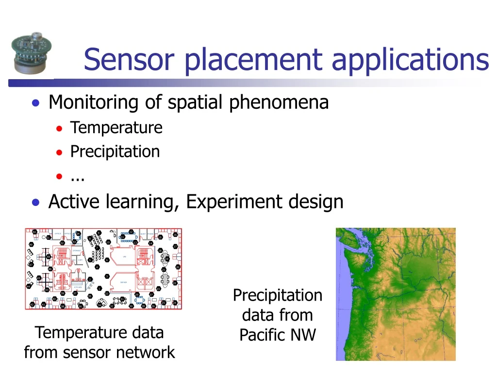
Precipitation data from Pacific NW Sensor placement applications • Monitoring of spatial phenomena • Temperature • Precipitation • ... • Active learning, Experiment design Temperature datafrom sensor network
This deployment: Evenly distributed sensors Sensor placement Chicken-and-Egg problem: No data or assumptions about distribution What’s the optimal placement? Don’t know where to place sensors
Becomes a covering problem Strong assumption – Sensing radius Problem is NP-complete But there are good algorithms with (PTAS) -approximation guarantees [Hochbaum & Maass ’85] Node predicts values of positions with some radius Unfortunately, approach is usually not useful… Assumption is wrong! For example…
Non-local, Non-circular correlations Complex, noisy correlations Individually, sensors are bad predictors. Rather: Noisy correlations! Circular sensing regions? Invalid: Complex sensing regions? Invalid:
Combining multiple sources of information • Combined information is more reliable • How do we combine information? • Focus of spatial statistics Temp here?
Uncertainty after observations are made more sure here less sure here Gaussian process (GP) - Intuition GP – Non-parametric; represents uncertainty; complex correlation functions (kernels) y - temperature x - position
Gaussian processes for sensor placement Posterior mean temperature Posterior variance Goal: Find sensor placement with least uncertainty after observations Problem is still NP-complete Need approximation
Entropy criterion (c.f., [Cressie ’91]) • A Ã; • For i = 1 to k • Add location Xi to A, s.t.: 3 4 1 Entropy High uncertainty given current set A – X is different 5 2 Uncertainty (entropy) plot 1 2 3 4 5
“Wasted” information Entropy criterion (c.f., [Cressie ’91]) Example placement Entropy criterion wastes information, Indirect, doesn’t consider sensing region – No formal guarantees
We propose: Mutual information (MI) • Locations of interest V • Find locations AµV maximizing mutual information: • Intuitive greedy rule: Uncertainty of uninstrumented locations before sensing Uncertainty of uninstrumented locations after sensing Low uncertainty given rest X is informative High uncertainty given A X is different
Temperature data placements: Entropy Mutual information Mutual information Intuitive criterion – Locations that are both different and informative Can we give guarantees about the greedy algorithm?
Decreasing Increasing with increasing A Important Observation • Intuitively, new information is worth less if we know more (diminishing returns) • Submodular set functions are a natural formalism for this idea: f(A[ {X}) – f(A) • Greedy rule proves that MI is submodular! B A {X} ¸ f(B [ {X}) – f(B) for A µ B
How can we leverage submodularity? • Theorem [Nemhauser et al ‘78]: The greedy algorithm guarantees (1-1/e) OPTapproximation for monotone SFs! • Same guarantees hold for the budgeted case [Sviridenko / Krause, Guestrin] • Unfortunately, I(V,{}) = I({},V) = 0,Hence MI in general is not monotonic! Locations can have different costs
Result of our algorithm Constant factor Optimal solution Guarantee for mutual information sensor placement Theorem: For fine enough (polynomially small) discretization, greedy MI algorithm provides constant factor approximation. For placing k sensors and >0:
Theorem: Mutual information sensor placement • Proof sketch • Nemhauser et al. ’78 theorem approximately holds for approximately non-decreasing submodular functions • For smooth kernel function, prove that MI is approximately non-decreasing if A is small compared to V • Quantify relation between A and V to guarantee that a discretization of suffices, where M is maximum variance per location, and σ is the measurement noise.
Efficient computation usinglocal kernels • Computation of the greedy rule requires computing where • This requires solving systems of N variables, time O(N3) with N locations to select from, total O(k N4) • Exploiting locality in covariance structure leads to an algorithm running in time for a problem specific constant d.
Deployment results Used initial deployment to select 22 sensors Learned new Gaussian process on test data using just these sensors All sensors Entropy selection MI selection Posterior mean Posterior variance Mutual information has 3 times less variance than entropy
Summary of Results • Proposed mutual information criterion for sensor placement in Gaussian processes • Exact maximization is NP-hard • Efficient algorithms for maximizing MI placements, strong approximation guarantee (1-1/e) OPT-ε • Exploitation of local structure improves efficiency • Compared to commonly used entropy criterion,MI placements provide superior prediction accuracy for several real-world problems.