Download

1 / 31
310 likes | 789 Views
Systems Reliability, Supportability and Availability Analysis. Systems Reliability Growth Planning and Data Analysis. Systems Reliability Growth Planning. The Duane Model. The instantaneous MTBF as a function of cumulative test time is obtained mathematically from MTBF C (t) and is given by

E N D
Systems Reliability, Supportability and Availability Analysis Systems Reliability GrowthPlanning and Data Analysis
The Duane Model The instantaneous MTBF as a function of cumulative test time is obtained mathematically from MTBFC(t) and is given by where MTBFi(t) is the instantaneous MTBF at time t and is interpreted as the equipment MTBF if reliability development testing was terminated after a cumulative amount of testing time, t.
Reliability Growth Factors Initial MTBF, K, depends on • type of equipment • complexity of the design and equipment operation • Maturity Growth rate, α • TAAF implementation and FRACAS Management • type of equipment • complexity of the design and equipment operation • Maturity
1000 Instantaneous MTBF 100 Cumulative 10 1000 10 100 10000 Cumulative Test Hours MTBF Growth Curves
The Duane Model The Duane Model may also be formulated in terms of equipment failure rate as a function of cumulative test time as follows: and where C(t) is the cumulative failure rate after test time t k* is the initial failure rate and k*=1/k, α is the failure rate growth (decrease rate) i(t) is the instantaneous failure rate at time t
Determination of Reliability Growth Test Time Specified MTBF at system maturity, θ0 Solve Duane Model for t
Determination of Reliability Growth Test Time - Example Determine required test time to achieve specified MTBF, θ0=1000, if α=0.5 and K=10 Solution
Determination of Reliability Growth Test Time – Example (continued) Interpretation of θ0=1000 hours at t=2499.88 hours If no further reliability growth testing is conducted, the systems failure rate at t=2499.88 hours is Failures per hour, and is constant for time beyond t=2499.88 hours
Determination of Reliability Growth Test Time Example (continued) Check since Cumulative MTBF at t = 2499.88 hours Since =1000 =500
Determination of Reliability Growth Test Time – Example Test Time Determine the test time required to develop (grow) the reliability of a product to 0 if the required reliability is 0.9 based on a 100-hour mission and the initial MTBF is 20% of 0 and =0.3. How many failures would you expect to occur during the test? Investigate the effect on the test time needed to achieve the required MTBF of deviations in initial MTBF and growth rate.
Determination of Reliability Growth Test Time Example (continued) The test time required depends on the starting point. The usual convention is to start the growth curve at t=100. We will determine the test time based on this. Also, we will show the effect on the requirement test time if the starting point of 0.20 is at t=1 hour. Required MTBF a=0.3 20% of Required MTBF Required Test Time 1 100 tR1 tR100
Determination of Reliability Growth Test Time – Example (continued) Since Using the Duane Model since =0.3
Determination of Reliability Growth Test Time – Example (continued) But and so that or so that the model is
Determination of Reliability Growth Test Time – Example (continued) To find the test time required to grow the MTBF to 0 set so that and
Determination of Reliability Growth Test Time – Example (continued) Since at t=21373.4 hours,
Determination of Reliability Growth Test Time – Example (continued) If the initial MTBFI(t) is interpreted to be at t=1 hour, then and so that or so that the model is
Determination of Reliability Growth Test Time – Example (continued) To find the test time required to grow the MTBF to 0 set so that and
Determination of Reliability Growth Test Time – Example (continued) Since at t=213.747 hours,
Reliability Growth Test Data Analysis Duane Model Parameter Estimation • Maximum Likelihood Estimation • Least Squares Estimation Plotting the estimated MTBF Growth Curves Procedures from MIL-HDBK-189, Feb. 13. 1981
Least Squares for the Duane Model Since MTBFc(t)=Kt, And for simplicity in the calculations, let: so that Transforming the data (ti, MTBFc(ti)) to (xi, yi) for i=1, 2, …, n use the method of least squares to estimate the equation y=0+ 1x+
Least Squares for the Duane Model Then the “best fit” Duane model is MTBFc(t)=Kt where k=e and α=b1 b0
Least Squares for estimating the Duane Model Parameter The Least squares estimates of 0 and 1 are:
Example - Reliability Growth Data Analysis A test is conducted to growth the reliability of a system. At the end of 100 hours of testing the results are as follows: tc MTBFC
Example - Reliability Growth Data Analysis - continued Estimate MTBFi(t)and MTBFc(t)as a function test time t and plot. What is the estimated MTBF of the system if testing is stopped at 200 hours?
Solution First plot the calculated cumulative MTBF values vs failure times MTBFC(t) MTBFi(t)
Solution Using the calculations from chart 27:
Solution At t=200 hours, the system failure rate becomes a constant ^ Failures per hour