Download
1 / 25
250 likes | 430 Views
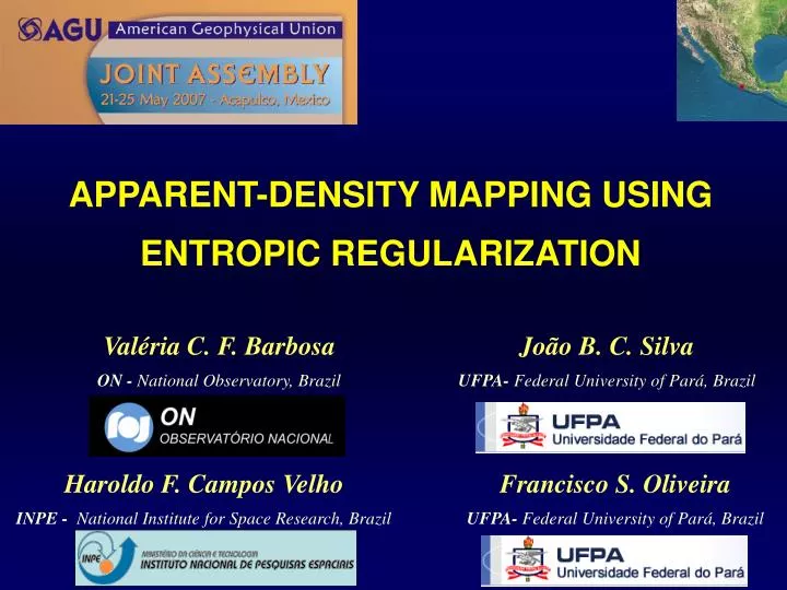
APPARENT-DENSITY MAPPING USING ENTROPIC REGULARIZATION. Valéria C. F. Barbosa ON - National Observatory, Brazil. João B. C. Silva UFPA- Federal University of Pará, Brazil. Haroldo F. Campos Velho INPE - National Institute for Space Research, Brazil. Francisco S. Oliveira

E N D
APPARENT-DENSITY MAPPING USING ENTROPIC REGULARIZATION Valéria C. F. Barbosa ON - National Observatory, Brazil João B. C. Silva UFPA- Federal University of Pará, Brazil Haroldo F. Campos Velho INPE - National Institute for Space Research, Brazil Francisco S. Oliveira UFPA- Federal University of Pará, Brazil
Contents Apparent-Density Mapping Using Entropic Regularization • Introduction and Objectives • Entropic Regularization Inversion • The Physical and Geologic Meaning of the Entropic Regularization • Synthetic Data Inversion Result • Real Data Inversion Result • Conclusions
2) Aerial and Satellite Photos Interpretation 1) Data Collection in the field 3) Geologic Interpretation Apparent-Density Mapping Using Entropic Regularization Introduction and Objectives The production of a geologic map includes:
y x Apparent-Density Mapping Using Entropic Regularization Introduction and Objectives The gravity method has been used as an auxiliary tool in geologic mapping to locate and delineate both outcropping and buried geological units and structures. It consists of estimating the spatial distribution of the density contrasts. Gupta and Grant (1985) Granser et al. (1989) Keating (1992)
y y mGal mGal mGal 1.4 0.6 x x y y y y 1.4 0.6 x x x x Apparent-Density Mapping Using Entropic Regularization Introduction and Objectives The elaboration of a geologic mapping using gravity data leads to solutions which despite being unique they are unstable. Apparent-density mapping is an ill-posed problem. A well-posed problem An ill-posed problem Tikhonov’s Regularization theory
Introduction and Objectives The Minimization of the First-Order Entropy The Maximization of the Zeroth-Order Entropy Prevents the estimated source to become an equivalent point source. Leads to solutions presenting more sharp borders Apparent-Density Mapping Using Entropic Regularization A new stable apparent-density mapping on the horizontal plane • Entropic Regularization
Methodology y Gravity Observations x o N g Î R z Interpretation Model 3D juxtaposed prisms 3D Gravity sources Estimate the 3D density-contrast distribution Apparent-Density Mapping Using Entropic Regularization
Methodology 2 1 h o - g g(p) = f N The problem of obtaining a vector of parameter estimates, p, that minimizes this functional is an ill-posed problem. ^ Apparent-Density Mapping Using Entropic Regularization The unconstrained Inverse Problem The linear inverse problem of estimating the density contrast, p, using just the gravity data, go, can be formulated by minimizing
Methodology Data misfit functional Nonnegative scalar First–order Tikhonov regularization functional Apparent-Density Mapping Using Entropic Regularization The traditional Inverse Problem A classic regularization method is solved by minimizing: 2 2 o = - + l ) F p ( g g(p) Rp 2 2 Introduce prior information that the spatial distribution of the density contrast is overall smooth Global Smoothness Inversion
[ Q ( p ) / Q ] [ Q ( p ) / Q ] minimize maximize 0 0 1 1 max max 2 o - g(p) g = d Apparent-Density Mapping Using Entropic Regularization Methodology The Entropic Regularization Inverse Problem The method estimates the constrained parameter by combining the maximum zeroth-order entropyand minimum first-order entropy measures of vector p and Subject to
Q where is normalizing constant and 0 max Q is based on the maximum entropy principle(Shannon and Weaver, 1949; Jaynes, 1957) 0 M + e ˆ p + e å ˆ p k = - k Q ( p ) log M M 0 å å + e ˆ = p k 1 + e ˆ p i i = 1 i = 1 i [ Q ( p ) / Q ] [ Q ( p ) / Q ] minimize maximize 0 0 1 1 max max where is normalizing constant and Q is based on the minimum entropy measureof the vector of first-order derivatives of p Q 1 (CamposVelho and Ramos, 1997; Ramos et al., 1999) 1 max M-1 å = - log Q ( p ) | | | | 1 ˆ ˆ p p - - + e + e ˆ ˆ p p = k 1 k k k+1 k+1 M -1 M -1 | | | | ˆ ˆ p p - - + e + e ˆ ˆ p p å å i i i+1 i+1 Apparent-Density Mapping Using Entropic Regularization = = i i 1 1 Methodology The Entropic Regularization Inverse Problem
and [ Q ( p ) / Q ] minimize 1 1 max Subject to 2 o - g(p) g = d [ Q ( p ) / Q ] maximize 0 0 max 2 t o p ( ) g Q ( p ) Q ( p ) - = go - g(p) g1 + 0 1 Q Q 2 0 max 1 max Methodology The Entropic Regularization Inverse Problem We solve this constrained inverse problem formulated as by minimizing the unconstrained functional: positive numbers called regularizing parameters
M + e ˆ p + e å ˆ p k = - k Q ( p ) Q log M M 0 0 å å + e ˆ = when all M prisms of the interpretation model have the same density-contrast estimate, i.e., p The maximum: k 1 + e ˆ p i i = 1 i = 1 i =c ˆ p M c c k M c c = log = log log ( M ) c c M M M M c å å c = Q ( p ) å å = 0 = 1 i - - 1 i The maximization of tends to maximize the smoothness of the spatial distribution of the density contrasts = = k k 1 1 Apparent-Density Mapping Using Entropic Regularization The Physical and Geologic Meaning of the Entropic Regularization • The zeroth-order entropy measure
Q The minimum: | | =c ˆ p Let us assume that nonnull differences - 1 ˆ p k k+1 Let us assume that D is the number of discontinuities between adjacent elements of density-contrast estimates, i.e., | | ≠ 0 ˆ p - ˆ p k k+1 D c c D c c = log = log log ( D ) = M-1 Q ( p ) c c D D å D D c å = - å c log Q ( p ) 1 | | | | 1 = = ˆ ˆ i 1 i 1 p p - - å å + e + e ˆ ˆ p p = k 1 - - k k k+1 k+1 M -1 M -1 | | | | ˆ ˆ p p = - - = + e + e k k 1 1 ˆ ˆ p p å å The minimization of tends to minimize the number of discontinuities in the apparent-density-contrast distribution. i i i+1 i+1 Apparent-Density Mapping Using Entropic Regularization = = i i 1 1 The Physical and Geologic Meaning of the Entropic Regularization • The First-Order Entropy Measure
The Physical and Geologic Meaning of the Entropic Regularization Estimated density-contrast distribution Apparent-Density Mapping Using Entropic Regularization The judicious combination of entropy measures favors an estimated density-contrast distribution presenting locally smoothregionsseparated byabrupt discontinuities.
Synthetic Tests Apparent-Density Mapping Using Entropic Regularization Silva et al. Figure 8 Apparent-density mapping results Global Smoothness Inversion Entropic Regularization Inversion X
Synthetic Data Example ) ) m m k k ( ( Fitted anomalies X X 0.35 0.30 0.25 Observed noise-corrupted gravity anomaly 0.20 0.05 0.15 0.25 0.35 0.45 0.55 0.15 0.10 0.05 Density contrast (g/cm3) Y (km) Density contrast (g/cm3) g/cm3 0.32 0.26 Flat-topped prismatic sources 0.3 g/cm³ 0.20 0.14 0.08 0.02 -0.04 Apparent-Density Mapping Results Global Smoothness Entropic Regularization 0.35 0.30 0.25 0.20 0.15 0.10 0.05 0.05 0.15 0.25 0.35 0.45 0.55 Y (km)
Real Test Apparent-Density Mapping Using Entropic Regularization Silva et al. Figure 8 Gravity data from the eastern Alps
Geological Map of part of the eastern Alps (Krainer 2002) 47o N 15o E 14o E Paleozoic of Graz Engadin Window Northern Calcareous Alps, Drau Range Radstätter Tauern Tertiary Basins Southern Alps Gurktal Nappe Crystalline Basement Rocks Major faults Apparent-Density Mapping Using Entropic Regularization Silva et al. Figure 8
Bouguer anomaly of part of the eastern Alps Granser et al. (1989) Apparent-Density Mapping Using Entropic Regularization Silva et al. Figure 8 28 22 47o N 16 10 4 -2 -8 14o E 15o E -14 mGal
Apparent-Density Mapping Results from the eastern Alps 47o N Fitted anomalies 47o N Bouguer anomaly 14o E 15o E 14o E 15o E 0.32 0.24 0.16 0.08 0 -0.08 -0.16 g/cm3 Global Smoothness Entropic Regularization Density contrast (g/cm3) Density contrast (g/cm3)
Conclusions Locally SmoothRegions Estimated density-contrast distribution Abrupt Discontinuities APPARENT-DENSITY MAPPING METHOD ENTROPIC REGULARIZATION INVERSION • Maximum zeroth-order entropy measure • Minimum first-order entropy measure
Apparent-Density Mapping Using Entropic Regularization Thank You I hope to see you in Rio de Janeiro at the Tenth International Congress of the Brazilian Geophysical Society ! November 19 - 23, 2007 Let us think about the Second Union-Wide Meeting in Latin America !
The iterative process stops 5.5 At the position where the discrete second difference of the objective function along the iterations changes its sign. 5.0 4.5 t(p) 4.0 3.5 3.0 0 4 8 12 16 20 Iteration