Download
1 / 52
650 likes | 1.16k Views
Multi-Criteria Decision Making by: Mehrdad ghafoori Saber seyyed ali. MCDM. PRESENTATION CONTENT:. MCDM definition Problem solving steps Criteria specifications Weighting the criteria Standardizing the raw scores Problem solving techniques. MCDM definitions.

E N D
Multi-Criteria Decision Makingby:Mehrdad ghafoori Saber seyyed ali MCDM
PRESENTATION CONTENT: • MCDM definition • Problem solving steps • Criteria specifications • Weighting the criteria • Standardizing the raw scores • Problem solving techniques
MCDM definitions - consists of constructing a global preference relation for a set of alternatives evaluated using several criteria - selection of the best actions from a set of alternatives, each of which is evaluated against multiple,and often conflicting criteria.
MCDM consists of two related paradigms: • MADM: these problems are assumed to have a predetermined , limited number of decision alternatives. • MODM: the decision alternatives are not given. instead the set of decision alternatives is explicitly defined by constraints using multiple objective programming. the number of potential decision alternatives may be large.
MCDM problem has four elements: • Goal • Objectives • Criteria • Alternatives
Examples of Multi-Criteria Problems • In determining an electric route for power transmission in a city, several criteria could be considered: • Cost • Health • Reliability • Importance of areas
Examples of Multi-Criteria Problems • Locating a nuclear power plant involves criteria such as: • Safety • Health • Environment • Cost
Problem solving steps: 1) Establish the decision context, the decision objectives (goals), and identify the decision maker(s). 2) Identify the alternatives. 3) Identify the criteria (attributes) that are relevant to the decision problem.
Problemsolving steps: 4) For each of the criteria, assign scores to measure the performance of the alternatives against each of these and construct an evaluation matrix (often called an options matrix or a decision table).
Problem solving steps: 5) Standardize the raw scores to generate a priority scores matrix or decision table. 6) Determine a weight for each criterion to reflect how important it is to the overall decision.
Problem solving steps: 7) Use aggregation functions (also called decision rules) to compute an overall assessment measure for each decision alternative by combining the weights and priority scores. 8) Perform a sensitivity analysis to assess the robustness of the preference ranking to changes in the criteria scores and/or the assigned weights.
Criteriacharacteristics • Completeness:It is important to ensure that all of the important criteria are included. • Redundancy:In principle, criteria that have been judged relatively unimportant or to be duplicates should be removed at a very early stage. • Operationality:It is important that each alternative can be judged against each criterion.
Criteria characteristics • Mutual independence of criteria: Straightforward applications of MCDM require that preferences associated with the consequences of the alternatives are independent of each other from one criterion to the next. • Number of criteria: An excessive number of criteria leads to extra analytical effort in assessing input data and can make communication of the results of the analysis more difficult.
Weighting the criteria: • Direct Determination • Rating, Point allocation, Categorization • Ranking • Swing • Trade-off • Ratio (Eigenvector prioritization) • Indirect Determination • Centrality • Regression – Conjoint analysis • Interactive
Weighting the criteria: -The ranking method: In this method, the criteria are simply ranked in perceived order Of importance by decision- makers: c1 > c2 > c3 > … > ci . The method assumes that the weights are non-negative and sum to 1. - Rating method: The point allocation approach is based on allocating points ranging from 0 to 100, where 0 indicates that the criterion can be ignored, and 100 represents the situation where only one criterion need to be considered. In ratio estimation procedure which is a modification of the point allocation method. A score of 100 is assigned to the most important criterion and proportionally smaller weights are given to criteria lower in the order. The score assigned for the least important attribute is used to calculate the ratios.
Weighting the criteria: - Pair wise comparison method: involves pair wise comparisons to create a ratio matrix. It uses scale table for pair wise comparisons and then computes the weights.
Standardizing the raw scores • Because usually the various criteria are measured in different units, the scores in the evaluation matrix S have to be transformed to a normalized scale. some methods are :
Problem solving techniques Some problem solving techniques are : • SAW (Simple Additive Weighting) • TOPSIS (Technique for Order Preference by Similarity to the Ideal Solution) • ELECTRE (Elimination et Choice Translating Reality) • BAYESIAN NETWORK BASED FRAMEWORK • AHP (The Analytical Hierarchy Process) • SMART (The Simple Multi Attribute Rating Technique ) • ANP (Analytic network process)
The selection of the models are based on the following evaluation criteria suggested by Dodgson et al. (2001): • internal consistency and logical soundness; • transparency; • ease of use; • data requirements are consistent with the importance of the issue being considered; • realistic time and manpower resource requirements for the analytical process; • ability to provide an audit trail; and • software availability, where needed.
SAW (Simple Additive Weighting): Multiplies the normalized value of the criteria for the alternatives with the importance of the criteria .the alternative with the highest score is selected as the preferred one.
A simple example of using SAW method • Objective • Selecting a car • Criteria • Style, Reliability, Fuel-economy • Alternatives • Civic Coupe, Saturn Coupe, Ford Escort, Mazda Miata
Weights and Scores Weight 0.3 0.4 0.3 Si Style Reliability Fuel Eco. 8.4 7.6 7.5 7.0 7 9 9 Civic Saturn 8 7 8 Ford 9 6 8 6 7 8 Mazda
TOPSIS(Technique for Order Preference by Similarity to the Ideal Solution) • In this method two artificial alternatives are hypothesized: • Ideal alternative: the one which has the best level for all attributes considered. • Negative ideal alternative: the one which has the worst attribute values. • TOPSIS selects the alternative that is the closest to the ideal solution and farthest from negative ideal alternative.
Input to TOPSIS • TOPSIS assumes that we have m alternatives (options) and n attributes/criteria and we have the score of each option with respect to each criterion. • Let xijscore of option iwith respect to criterion j We have a matrix X = (xij) mn matrix. • Let J be the set of benefit attributes or criteria (more is better) • Let J' be the set of negative attributes or criteria (less is better)
Steps of TOPSIS • Step 1: Construct normalized decision matrix. • This step transforms various attribute dimensions into non-dimensional attributes, which allows comparisons across criteria. • Normalize scores or data as follows: rij = xij/ √(x2ij) for i = 1, …, m; j = 1, …, n i
Steps of TOPSIS • Step 2: Construct the weighted normalized decision matrix. • Assume we have a set of weights for each criteria wj for j = 1,…n. • Multiply each column of the normalized decision matrix by its associated weight. • An element of the new matrix is: vij = wj rij
Steps of TOPSIS • Step 3: Determine the ideal and negative ideal solutions. • Ideal solution. A* = { v1*, …, vn*}, where vj*={ max (vij) if j J ; min (vij) if j J' } ii • Negative ideal solution. A' = { v1', …,vn' }, where v' = { min (vij) if j J ; max (vij) if j J' } ii
Steps of TOPSIS • Step 4: Calculate the separation measures for each alternative. • The separation from the ideal alternative is: Si *= [ (vj*– vij)2 ] ½ i = 1, …, m j • Similarly, the separation from the negative ideal alternative is: S'i = [ (vj' – vij)2 ] ½ i = 1, …, m j
Steps of TOPSIS • Step 5: Calculate the relative closeness to the ideal solution Ci* Ci*= S'i / (Si* +S'i ) ,0 Ci* 1 Select the Alternative with Ci* closest to 1.
An example of using TOPSIS method Weight 0.1 0.4 0.3 0.2 Reliability Fuel Eco. Style Cost Civic 7 9 9 8 Saturn 8 7 8 7 9 6 8 9 Ford 678 6 Mazda
Steps of TOPSIS • Step 1: calculate (x2ij )1/2 for each column and divide each column by that to get rij Style Rel. Fuel Cost Civic 0.46 0.61 0.54 0.53 Saturn 0.53 0.48 0.48 0.46 Ford 0.59 0.41 0.48 0.59 0.40 0.48 0.48 0.40 Mazda
Steps of TOPSIS • Step 2 : multiply each column by wj to get vij. Style Rel. Fuel Cost 0.046 0.244 0.162 0.106 Civic Saturn 0.053 0.192 0.144 0.092 Ford 0.059 0.164 0.144 0.118 0.040 0.192 0.144 0.080 Mazda
Steps of TOPSIS Step 3 (a): determine ideal solution A*. A* = {0.059, 0.244, 0.162, 0.080} Style Rel. Fuel Cost Civic 0.046 0.244 0.162 0.106 Saturn 0.053 0.192 0.144 0.092 Ford 0.0590.164 0.144 0.118 0.040 0.1920.144 0.080 Mazda
Steps of TOPSIS Step 3 (b): find negative ideal solution A'. A' = {0.040, 0.164, 0.144, 0.118} Style Rel. Fuel Cost Civic 0.046 0.244 0.162 0.106 Saturn 0.053 0.192 0.144 0.092 Ford 0.059 0.164 0.144 0.118 0.040 0.1920.144 0.080 Mazda
Steps of TOPSIS Step 4 (a): determine separation from ideal solution A* = {0.059, 0.244, 0.162, 0.080} Si*= [ (vj*– vij)2 ] ½for each row j Style Rel. Fuel Cost Civic (.046-.059)2 (.244-.244)2(0)2(.026)2 Saturn (.053-.059)2 (.192-.244)2(-.018)2(.012)2 Ford (.053-.059)2 (.164-.244)2(-.018)2 (.038)2 Mazda (.053-.059)2 (.192-.244)2(-.018)2 (.0)2
Steps of TOPSIS Step 4 (a): determine separation from ideal solution Si* (vj*–vij)2 Si*= [ (vj*– vij)2 ] ½ Civic 0.000845 0.029 Saturn 0.003208 0.057 Ford 0.008186 0.090 Mazda 0.003389 0.058
Steps of TOPSIS Step 4: determine separation from negative ideal solution Si' Si' = [ (vj'– vij)2 ] ½ (vj'–vij)2 Civic 0.006904 0.083 Saturn 0.001629 0.040 Ford 0.000361 0.019 Mazda 0.002228 0.047
Steps of TOPSIS Step 5: Calculate the relative closeness to the ideal solution Ci*= S'i / (Si* +S'i ) S'i /(Si*+S'i) Ci* Civic 0.083/0.112 0.74 BEST Saturn 0.040/0.097 0.41 Ford 0.019/0.109 0.17 Mazda 0.047/0.105 0.45
AHP (The Analytical Hierarchy Process) • AHP uses a hierarchical structure and pairwise comparisons. • An AHP hierarchy has at least three levels: 1) the main objective of the problem at the top. 2) multiple criteria that define alternatives in the middle.(m) 3) competing alternatives at the bottom.(n)
Steps of AHP • Criteria weighting must be determined using (m*(m-1))/2 pair wise comparisons. • Alternatives scoring using m*((n*(n-1))/2) pair wise comparisons between alternatives for each criteria. • After completing pair wise comparisons AHP is just the hierarchical application of SAW.
Some AHP method shortcomings • Comparison inconsistencies: decision-makers using AHP often make inconsistent pair wise comparisons. • Rank reversals changing of relative alternative rankings due to the addition and deletion of alternatives. • Large number of comparisons where there are either a large number of attributes and/or alternatives to be evaluated.
SMART(The Simple Multi Attribute Rating Technique ) • In a general sense, SMART is somewhat like AHP in that a hierarchical structure is created to assist in defining a problem and to organize criteria. However, there are some significant differences between two techniques: 1) SMART uses a different terminology. For example, in SMART the lowest level of criteria in the value tree (or objective hierarchy) are called attributes rather than sub-criteria and the values of the standardized scores assigned to the attributes derived from value functions are called ratings.