Download
1 / 19
190 likes | 294 Views
Dynamics. Vorticity In the previous lecture, we used “scaling” to simplify the equations of motion and found that, to first order, horizontal winds are geostrophic while, in the vertical, the system is “static” (i.e. hydrostatic)

E N D
Dynamics • Vorticity • In the previous lecture, we used “scaling” to simplify the equations of motion and found that, to first order, horizontal winds are geostrophic while, in the vertical, the system is “static” (i.e. hydrostatic) • This does not imply that there are no vertical motions, just that these vertical motions are not driven by vertical pressure gradients • One of the limitations of the geostrophic approximation, however, is that it does not allow us to predict the evolution of the system because there is no term that is related to the time rate of change • In order to include the time rate of change of the winds, we need to look at scaling associated with the next order of magnitude
Dynamics • Vorticity • If we now keep all terms of order 10-4and 10-5, the horizontal equations become: (Eqn.) • We take the “curl” of these two equations by taking the x-derivative of the meridional wind equation and the y-derivative of the zonal wind equation, and then subtract the two (Eqn.) • We can now define the “relative vorticity” as: (Eqn.) • By this definition, cyclonic circulation is defined to have positive relative vorticity, while anti-cyclonic circulation is defined to have negative relative vorticity
Dynamics • Vorticity • Putting the definition for vorticity into the pervious equation gives: (Eqn.) • From before, we write the the hydrostatic equation as: (Eqn.) • We can define the “height” of a given pressure level as (x,y,t): (Eqn.) • If we then integrate the hydrostatic equation with depth and use the conservation of mass we find that: (Eqn.)
Dynamics • Vorticity • We can put this equation into the previous equation for vorticity: (Eqn.) • Finally, assume H>> : (Eqn.) • This equation is called the “Conservation of Potential Vorticity”
Dynamics • Vorticity • New term in the vorticity equation is “Planetary vorticity” • From before, we defined the Coriolis parameter as: (Eqn.) • We can approximate this dependence as: (Eqn.) • Using this “Beta approximation”, the Coriolis parameter can be written as: (Eqn.)
Dynamics • Vorticity • Putting this approximation into the potential vorticity equation gives: (Eqn.) • Only holds following the path of given air parcel • To simplify a bit more, we add two approximations: • H>> • fo~10-4; by~10-5 • Using these approximations, it can be shown that: (Eqn.)
Dynamics • Vorticity • Ex.1 Lee-side low pressures • Typically we find that low pressures tend to form on the lee-side of mountains • This can be seen in daily weather maps as well as in the general circulation of the atmosphere • Ex.2 Planetary waves • In the large-scale circulation, it is possible to find wave-like patterns that are fairly stationary or move only very slowly • We can understand the dynamics of these waves by looking at the behavior of an air parcel that is initially moving to the north • As with the lee-side low, these features can be seen both in the daily fields as well as the climate fields
Dynamics • Vorticity • Waves of this kind are called “planetary” or “Rossby” waves. • Short Rossby waves • Long Rossby waves • Short Rossby waves • a balance between planetary vorticity and relative vorticity, as described above • Long Rossby waves • a balance between planetary vorticity and height • This produces global-scale wave-like features seen earlier
Dynamics • Vorticity
Dynamics • Vorticity
Dynamics • Vorticity
Dynamics • Vorticity
Dynamics • Vorticity
Dynamics • Vorticity
Dynamics • Vorticity
Dynamics • Vorticity
Dynamics • Vorticity Z E N L H E
Dynamics • Vorticity
Dynamics • Vorticity