Cutting-Edge Global Nonhydrostatic Modelling Techniques

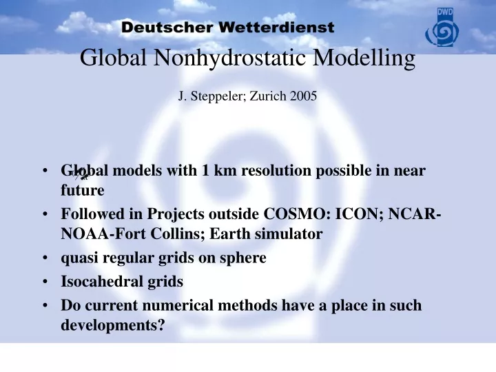
1. Global Nonhydrostatic ModellingJ. Steppeler; Zurich 2005 • Global models with 1 km resolution possible in near future • Followed in Projects outside COSMO: ICON; NCAR-NOAA-Fort Collins; Earth simulator • quasi regular grids on sphere • Isocahedral grids • Do current numerical methods have a place in such developments?

2. Desirable features of discretisations on the sphere • Nonhydrostatic • Accuracy: Order 3 or higher in space [and time] • (Observation of approximation conditions: smoothness ( for third order schemes), Smooth physics interface, smooth orography (dh<dz) or z-coordinate) • Conservation: mass, energy • Efficiency (computer time and development time) • (Positivity of advection: flux correction) • (Nesting option: Skamarock method) • Ability to incorporate developments for nh models

3. The Baumgardner principle(Rules of good behaviour on triangelsProven for o2, not yet for o3Supported by the success of Skamarock nesting) • No global coordinate • Keep approximation order at grid interfaces • The faithful are rewarded by having no problems carrying plane discretisations to the sphere

4. Quasi regular grids • Structured (index i,j) • Each line of points j,i j,i+1 j,i+2............ is on a great circle • Obtained by projecting bilinear grids to the sphere • Projection of any vector r to the sphere with image ra:

5. Bilinear grids • Four points r1,r2,r3,r4 may have any position in space • Divide the sides of the rhomboid equally and connect opposite points • Bilinear grid theorem: each coordinate line intersects each line of the crossing coordinate line family. The grid is regular in each direction.

6. Orange cut grids • NP=3 NP=4 NP=5

7. Grid Stencils Baumgardner • Edges grid Edges grid • Order3 Order 2 Redundancy 19:9 Redundancy 6:5 or 5:5

8. Grid Stencils Baumgardner • Area grid Area grid • Order3 Order 1 (Finite Volume) Redundancy 13:9 Redundancy 4:3

9. Great Circle Grid Stencils • Edges grid • Order 3 • Local coordinate, for example local geographic • Possibility 1: irregular, but locally nearly regular grid Non orthogonal grid • Possibility 2: Rooftile grid: regular and nearly orthogonal

10. Interpolation • Grid redundancy is an issue for all methods relying on interpolation • Cascade interpolation for regular grids • Serendipidity interpolation: the part going into 2d and 3d look like linear. • Serendipidity grids replace forecasts of some points by order consistent interpolation

11. Discretisation Options, Based on Interpolation • Finite Volumes: Bonaventura choice, best on regularised grids, conservation possible, often low order, tested by Ringler and Steppeler • Baumgardner: suitable for somewhat irregular grids, tested for order 2 • Baumgardner Order2: Amplitudes on edges; small grid redundancy • Baumgardner Order3: Amplitudes on triangle surfaces, very irregular grid for plane waves, yet untested, (some grid redundancy) • Great circle grids: very similar to limited area discretisations, order 2,3 easily possible, RK, SI, SL, adaptation of all local developments easy (grid redundancy no problem) • Tiled grids: very uniform grids (~1%), less elegant look, spectral elements possible) • Serendipidity grids (can be derived as a further development of SE)

12. Saving factors of Discretisations • Finite Volumes: 1 • Baumgardner Order2: 1 • Baumgardner Order3: 1 • Great circle grids: RK, SI, SL 1 now 3 seem possible • Tiled grids: 1.5 • Serendipidity grids 3 • Unstructured • Conservation

13. Dual grid and conservation • Use conservation form, compute fluxes • 1st possibility: WRF-method • 2nd: Flux correction • Issue: order of representation of the conserved quantity

14. Third order scheme on sphere, symmetric water wave