An Analytical Approach to Studying Non-exponential Decay

1. An Analytical Approach to Studying Non-exponential Decay Athanasios Petridis Drake University COLLABORATORS: L. Staunton (Drake Univ.) M. Luban (Iowa State Univ.) J. Vermedahl (Drake Univ.)

2. Outline • Introduction to the Problem • An Analytical Approach • Infinite Wall and Delta-function Potential • Even Potentials • Statistical Behavior • Conclusions and Perspectives

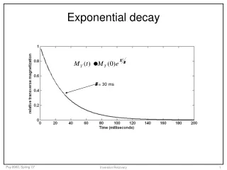
3. Introduction to the Problem • It is generally expected that wavefunctions initially set inside potential wells will decay exponentially if they are not eigenfunctions. • The Breit-Wigner energy distribution leads to exponential decay of resonances. • Numerical studies of the time-dependent Schrödinger equation show that this is not generally true.

4. x L Harmonic oscillator (HO) potential “cut” at one classical amplitude with the HO ground state as the initial function. V 0

5. The survival probability, Pin, decreases following a “median” function that is non-exponential at small times and on which there are superimposed oscillations.

6. An Analytical Approach • Solve the time-independent Schrödinger equation subject to boundary conditions to obtain . • Use completeness for the given Hilbert space and locality to obtain time-dependent solutions: • The spectral function, (E), must yield convergent energy (E) integrals and square-integrable wavefunctions for all times.

7.   V0(x-L) (I) (II) 0 L x Infinite Wall and Delta-function Potential With the choice: the energy integrals converge and  is normalizable

8. II (x,t) = Time-dependent solutions in the two regions (L = 3). I (x,t) =

9. Snapshots of the probability density at various times C A K = 0.5 D B NOTE: No ripples in region (I) due to odd solution

10. Pin(t) = The survival probability is NOT a simple exponentially decaying function The probability to find the particle “outside” is verified to be the exact complement of Pin(t).

11. The survival probability versus time The probability to find the particle “outside” versus time.

12.   (II-) (I) (II+) -L 0 +L x Even Potentials V NOTE: In all three regions waves propagating in both directions are acceptable solutions. The energy eigenfunctions need not have definite parity even in region (I). A and B are independent.

13. Sine and Cosine solutions project out parts of the spectral function which are even or odd in the momentum (p). Their coefficients may differ. • We consider the solution as a superposition of “incoming” and “outgoing” plane waves; e.g. in region (I):

14. In the case of overall even symmetry in x we select the “incoming” wave spectral function to have one or more poles with negative imaginary part: (outgoing) (incoming)

15. The integral that includes the pole is done with contour integration and using the residue theorem. The negative imaginary part ensures that the wavefunction dies-out at large distances. • The other integral is also convergent and yields a square-integrable function as well. • The probability density has an oscillatory cross-term.

16. Probability density in region (I) for x > 0 at various times (L = 1) A C B D E0 = 20, 0 = 1, K = 0.5

17. ½ of the survival probability versus time (x >0). Detail of the above plot: non-exponential median with superimposed oscillations of decaying amplitude.

18. Statistical Behavior • At large times the survival probability decays essentially like an exponential. • For many-particle systems the “starting time” for the decay is not the same for all members. • Therefore, there is smearing of the observed deviations from exponential decay (work in progress).

19. Conclusions and Perspectives • Non-exponential decay of wavefunctions has been established ANALYTICALLY and NUMERICALLY (presentation by Jon Vermedahl). • The details depend on the potential and the spectral function. • Extension to many (independent) particle systems is under-way.