Download
1 / 23
250 likes | 394 Views
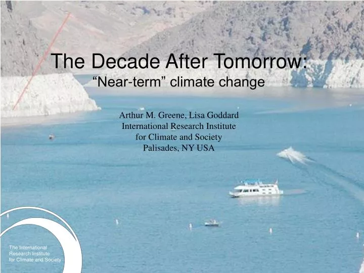
The Decade After Tomorrow: “Near-term” climate change Arthur M. Greene, Lisa Goddard International Research Institute for Climate and Society Palisades, NY USA. The International Research Institute for Climate and Society. Outline. “Near-term” climate change: What is it?

E N D
The Decade After Tomorrow: “Near-term” climate changeArthur M. Greene, Lisa GoddardInternational Research Institutefor Climate and SocietyPalisades, NY USA The International Research Institute for Climate and Society
Outline • “Near-term” climate change: What is it? • Large-scale modes of variability: What are they? • Near- and far-field effects: Maybe in my backyard • Value in paleorecords: Characterize, if not predict… • Prediction: The wave of the future The International Research Institute for Climate and Society
Why “Near-term?” • Interest in regional climate change is increasing, but the 100-year time scales considered by IPCC are often deemed too long to be “actionable.” Thus is born the concept of “near-term climate change” – out to about three decades. • But there’s a catch: Decadal variability is much lesswell-understood than, say, ENSO. It may even originate from completely random interactions between atmosphere and ocean. The International Research Institute for Climate and Society ENSO: El Niño-Southern Oscillation
“Near-term” prediction in context SI forecast / verification “Near-term CC” IPCC “climate change” time scale SI: Seasonal-to-Interannual (ENSO-based) IPCC: Intergovernmental Panel on Climate Change Aside: Observational datasets are not all identical The International Research Institute for Climate and Society
Animation: http://www.phy.ntnu.edu.tw/ntnujava/index.php?topic=24 Atmosphere-ocean randomness: Brownian motion Path of the (massive) red object is smoother, and evolves more slowly, than those of the rapidly fluctuating grey “molecules.” The International Research Institute for Climate and Society
Decadal complexity Unlike in the case of ENSO, where a single, fairly well-understood mechanism controls the evolution of events, the physical processes that produce decadal climate fluctuations differ from ocean basin to basin; there is no single dominant process. The processes themselves are generally not well-understood, nor is the degree to which they may interact. The International Research Institute for Climate and Society
Principal mode in the Atlantic: AMV (Atlantic Multidecadal Variability) Gray et al, 2004 Density-driven “Overturning” circulation • “Oscillation” vs “Variability”: The reconstruction suggests less regularity than might be inferred from the instrumental record alone. • Colored line (middle plot) can be thought of as the slowly varying path of the red “Brownian” object. T D -- Circulation slows, temperature falls. T D -- Circulation increases, temperature rises. Result: A natural oscillation Complication: Salinity
AMV far-field effects on rainfall, in observations and models Decadal correlation maps for AMV and mean annual precipitation for (a) observations and picntrl runs for (b) GFDL-CM2.0, (c) GISS-ER and (d) NCAR-CCSM3.0
AMV effects on Atlantic hurricanes “During warm phases of the AMO, the numbers of tropical storms that mature into severe hurricanes is much greater than during cool phases, at least twice as many.” • Two 24-yr periods compared • Green lines: Tropical storms • Red lines: Hurricanes Worth keeping in mind: Other possible influences on Atlantic hurricanes are not taken into account here. But the research argument is in fact supported on basic physical grounds as well. Goldenberg et al., 2004
Pacific decadal variability: the PDO • First identified in a research paper about Salmon production. • Expressed as a pattern, where SST in the tropical Pacific varies out of phase with higher latitudes. “Warm” phase is shown at left. • Accompanied by changes in winds (arrows), SLP. • Teleconnections affect precipitation in many regions around the globe. • Cause is presently not understood; decadal variations in ENSO may play a role (pattern similarity). (Source: http://jisao.washington.edu/pdo)
PDO far-field effects on rainfall Scale: Amount (mm/day) by which rainfall changes for a 1-unit increase in the PDO index.
- PDO +AMO All together, now… AMO/PDO combined effects on drought Periods when these conditions applied McCabe et al, 2004 Recent states The International Research Institute for Climate and Society
Value of paleodata: Tree-ring reconstruction of PDSI in the Western U.S. Stahle et al., 2007 Red arrow: Date of the Colorado Water Compact (1922) Blue line: Portion of record used to estimate flows. The International Research Institute for Climate and Society
If they had known then what we know now…what? “In short, the river is allocated to the tune of 17.5 MAF (million acre-feet) … whereas the observed average yield is 14.8 MAF (1896-2004), and tree-ring reconstructions suggest a longer-term average yield of 13.5 MAF (1520-1961).” – Hard Times on the Colorado River: Growth, Drought and the Future of the Compact, 2005. Natural Resources Law Center, University of Colorado School of Law Level in 2002 (Lake Mead) Ken Dewey, HPRCC (U. Nebraska) The International Research Institute for Climate and Society
Important to keep in mind: Natural variability is only part of the picture! “If these models are correct… levels of aridity of the recent multiyear drought… will be-come the new climatology of the American Southwest within a time frame of years to decades.” – Seager et al., 2007
So what about prediction? • Since the long-term “memory” of the climate system must reside in the ocean, it is initialization of the model ocean that holds the key to decadal prediction. However: • Subsurface ocean observations are sparse, except for the past few years. This limits the accuracy with which models can be initialized and “hindcasts” can be verified. • Dynamical models currently do not do a very good job of simulating the observed space-time variability of the large-scale decadal modes. • Statistical prediction, which depends neither on subsurface ocean data nor dynamical model simulations, may be possible: This is an active area of research. The International Research Institute for Climate and Society
Model ensemble members limn the range of natural variability… Mean annual Atlantic SST, ensemble of simulations using GFDL-CM2.1, for SRES A1B. Ensemble members differ only in the initial conditions utilized, indicating range of internal variability. Heavy black line is ensemble mean; values are relative to 1991-2000. The International Research Institute for Climate and Society
Sampling the subsurface ocean: The ARGO program Positions of ARGO floats that have delivered data within the past 30 days. (http://www.argo.ucsd.edu/) The International Research Institute for Climate and Society
Dynamical prediction: State of the art Ten-year forecast beginning June 2005 (white line, red uncertainty bounds) and two 10-year hindcasts, beginning 1985, 1995. Blue line represents uninitialized forecasts; black line, observations (HADCRUT2v). (Smith et al., Science, 2007). Improvements in hindcast RMSE (9-year means) due to ocean initialization: A, B, C, surface temperature anomaly; D upper ocean heat content anomaly. The International Research Institute for Climate and Society
Statistical prediction: SST in the Southeast Asia domain Forced and natural signals are separated; each is then projected forward in time…
Forced and natural projections combined Not shown here, but important: Uncertainty envelope
Summary • Decadal climate variations have received increasing attention of late: • Possibly more relevant for adaptation than 100-year projections. • Less is known about underlying physical processes at this time scale. • Centennial, “IPCC-type” trends are not perforce irrelevant! • At least some decadal variability is associated with large-scale intrinsic modes. (Random atmosphere-ocean interaction may also play a role.) • Atlantic Multidecadal Variability (AMV or AMO) • Pacific Decadal Oscillation (PDO) • NAO, AO, NAM, SAM, PNA… • Teleconnections to many parts of globe • Physics relatively poorly understood; so far, not well modeled (by GCMs) • Paleorecords may aid in characterizing regional decadal variations of the past. • Tree-ring reconstructions • Corals, other paleoproxies • Potential utility for decision-making • Both dynamical and statistical forecasts may be possible: • Potential predictability, forecast skill, will vary from region to region. • Dynamical prediction depends on ocean initialization, since climate “memory” resides in the oceans. • Statistical forecasts (of the type discussed) decompose the signal, project components separately, recombine: Voilà, the “wave” of the future!
Thank you! amg@iri.columbia.edu