Download

1 / 60
600 likes | 753 Views
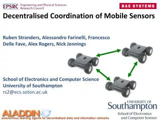
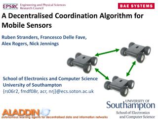
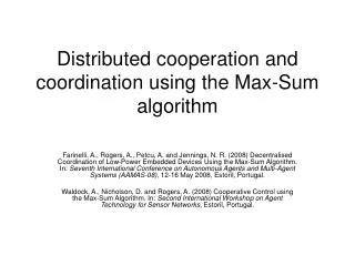
Decentralised Coordination of Mobile Sensors using the Max-Sum Algorithm. Ruben Stranders , Alessandro Farinelli , Alex Rogers, Nick Jennings. School of Electronics and Computer Science University of Southampton {rs06r2, af2, acr , nrj }@ ecs.soton.ac.uk.

E N D
Decentralised Coordination of Mobile Sensors using the Max-Sum Algorithm • Ruben Stranders, Alessandro Farinelli, Alex Rogers, Nick Jennings School of Electronics and Computer Science University of Southampton {rs06r2, af2, acr, nrj}@ecs.soton.ac.uk
This presentation focuses on the use of Max-Sum to coordinate mobile sensors Decentralised Control using Max-Sum Problem Formulation Model Value Coordinate Sensor Architecture
The key challenge is to monitor a spatial phenomenon with a team of autonomous sensors Sensors
The key challenge is to monitor a spatial phenomenon with a team of autonomous sensors • Limited • Communication
The key challenge is to monitor a spatial phenomenon with a team of autonomous sensors • No centralisedcontrol
Spatial phenomena are modelled as a spatial field over two spatial and one temporal dimensions
The aim of the sensors is to collectively minimise predictive uncertainty of the spatial phenomenon Predictive Uncertainty Contours
The main challenge is to coordinate the sensors in order to the state of these spatial phenomena • How to move • to minimise • uncertainty?
To solve this coordination problem, we had to address three challenges How to modelthe phenomena? How to value potential samples? How to coordinateto gather samples of highest value?
The three central challenges are clearly reflected in the architecture of our sensing agents Incoming negotiation messages Samples received from neighbouring agents Sensing Agent Value of potential samples Information processing Samples from own sensor Model Value Action Selection Model of Environment Coordinate Move Raw samples Outgoing negotiation messages Samples sent to neighbouring agents
These three challenges are clearly reflected in the architecture of our sensing agents Incoming negotiation messages Samples received from neighbouring agents Sensing Agent Value of potential samples Information processing Samples from own sensor Action Selection Model of Environment Move Raw samples Model Outgoing negotiation messages Samples sent to neighbouring agents
The sensors model the spatial phenomenon using the Gaussian Process Spatial Correlations Weak Strong
The sensors model the spatial phenomenon using the Gaussian Process Temporal Correlations Weak Strong
The value of a sample is determined how much it reduces uncertainty Incoming negotiation messages Samples received from neighbouring agents Sensing Agent Value of potential samples Information processing Samples from own sensor Action Selection Model of Environment Move Raw samples Value Outgoing negotiation messages Samples sent to neighbouring agents
The value of a sample is based on how much it reduces uncertainty • But how to determine uncertainty reduction before collecting a sample?
The value of a sample is based on how much it reduces uncertainty • But how to determine uncertainty reduction before collecting a sample? Prediction Confidence Interval Collected Sample Gaussian Process not only gives predictions, but also confidence intervals
The value of a sample is based on how much it reduces uncertainty Potential Sample Location • But how to determine uncertainty reduction before collecting a sample? Prediction Confidence Interval Collected Sample Gaussian Process not only gives predictions, but also confidence intervals
The value of a sample is based on how much it reduces uncertainty Measure of uncertainty • But how to determine uncertainty reduction before collecting a sample? Prediction Confidence Interval Collected Sample Gaussian Process not only gives predictions, but also confidence intervals
The value of a sample is based on how much it reduces uncertainty Specifically, we use Entropy , as information metric Prediction Confidence Interval Collected Sample
The sensor agents coordinate using the Max-Sum algorithm Incoming negotiation messages Samples received from neighbouring agents Sensing Agent Value of potential samples Information processing Samples from own sensor Action Selection Model of Environment Move Raw samples Coordinate Outgoing negotiation messages Samples sent to neighbouring agents
Using the Entropy criterion, the sum of the conditional values equals the team utility
The key problem is to maximise the social welfare of the team of sensors in a decentralised way Mobile Sensors Social welfare:
The key problem is to maximise the social welfare of the team of sensors in a decentralised way Variables Encode Movement
The key problem is to maximise the social welfare of the team of sensors in a decentralised way Utility Functions (These encode information value)
The key problem is to maximise the social welfare of the team of sensors in a decentralised way Localised Interaction
We can now use Max-Sum to solve the social welfare maximisation problem Optimality Complete Algorithms DPOP OptAPO ADOPT Max-Sum Algorithm Iterative Algorithms Best Response (BR) Distributed Stochastic Algorithm (DSA) Fictitious Play (FP) Communication Cost
The input for the Max-Sum algorithm is a graphical representation of the problem: a Factor Graph Variable nodes Function nodes Agent 3 Agent 1 Agent 2
Max-Sum solves the social welfare maximisation problem by local computation and message passing Variable nodes Function nodes Agent 3 Agent 1 Agent 2
Max-Sum solves the social welfare maximisation problem by local computation and message passing From variableito function j • From function j to variable i
To use Max-Sum, we encode the mobile sensor coordination problem as a factor graph Sensor 1 Sensor 2 Sensor 3 Sensor 1 Sensor 2 Sensor 3
Unfortunately, the straightforward application of Max-Sum is too computationally expensive From variableito function j From function j to variable i
Unfortunately, the straightforward application of Max-Sum is too computationally expensive From variableito function j From function j to variable i Bottleneck!
Therefore, we developed two general pruning techniques that speed up Max-Sum Goal: Make as small as possible
Therefore, we developed two general pruning techniques that speed up Max-Sum Goal: Make as small as possible Try to prune the action spaces of individual sensors Try to prune joint actions
The first pruning technique prunes individual actions by identifying dominated actions
The first pruning technique prunes individual actions by identifying dominated actions ↑ [1, 2] ↓ [3, 4] 1. Neighbours send bounds ↑ [2, 2] ↓ [1, 1] ↑ [5, 6] ↓ [0, 1]
The first pruning technique prunes individual actions by identifying dominated actions ↑ [1, 2] ↓ [3, 4] 2. Bounds are summed ↑ [2, 2] ↓ [1, 1] ↑ [5, 6] ↓ [0, 1] ↑ [8, 10] • ↓ [4, 7]
The first pruning technique prunes individual actions by identifying dominated actions 2. Bounds are summed ↑ [8, 10] • ↓ [4, 7]
The first pruning technique prunes individual actions by identifying dominated actions 3. Dominated actions are pruned X ↑ [8, 10] [8, 10] • ↓ [4, 7] [4, 7]
We developed two general pruning techniques that speed up Max-Sum Goal: Make as small as possible ✔ Try to prune the action spaces of individual sensors Try to prune joint actions
The second pruning technique reduces the joint action space because exhaustive enumeration is too costly Sensor 1 Sensor 2 Sensor 3
The second pruning technique reduces the joint action space because exhaustive enumeration is too costly Sensor 1 Sensor 2 Sensor 3
The second pruning technique reduces the joint action space because exhaustive enumeration is too costly Sensor 1 Sensor 2 Sensor 3
The second pruning technique reduces the joint action space because exhaustive enumeration is too costly
The second pruning technique prunes the joint action space using Branch and Bound Sensor 1 Sensor 2 Sensor 3
The second pruning technique prunes the joint action space using Branch and Bound Sensor 1 [0, 4] [7, 13] [2, 6] Sensor 2 Sensor 3
The second pruning technique prunes the joint action space using Branch and Bound Sensor 1 X X [0, 4] [7, 13] [2, 6] Sensor 2 Sensor 3
The second pruning technique prunes the joint action space using Branch and Bound Sensor 1 X X [0, 4] [7, 13] [2, 6] Sensor 2 9 10 7 8 Sensor 3
The second pruning technique prunes the joint action space using Branch and Bound Sensor 1 X X [0, 4] [7, 13] [2, 6] Sensor 2 O X X X 9 10 7 8 Sensor 3
This demonstration shows four sensors monitoring a spatial phenomenon