Download
1 / 30
300 likes | 547 Views
Two Temperature Non-equilibrium I sing Model in 1D . Nick Borchers. Outline. Background Non-equilibrium vs. Equilibrium systems Master e quation and Detailed Balance Ising model Preliminary Results Model description Dependence on external temperature

E N D
Two Temperature Non-equilibrium Ising Model in 1D Nick Borchers
Outline • Background • Non-equilibrium vs. Equilibrium systems • Master equation and Detailed Balance • Ising model • Preliminary Results • Model description • Dependence on external temperature • Dependence on infinite temperature region size • Dependence of lattice size • Future pursuits • Configuration Space characteristics and trajectories • Localized quantities and subsystems • Applications to living systems
Non-equilibrium versus equilibrium Equilibrium System Features: • Probability proportional to Boltzmann factor: • ‘Time Reversal’ Symmetry, or ‘Detailed Balance’
Steady-State vs. Equilibrium • Equilibrium is a special case of steady-statein which there is no steady flux through the system. This requires an isolated system, which is an idealization which must be carefully constructed. • There may be Non-Equilibrium Steady States (NESS), in which the inputs and outputs of the system are balanced, but there is a flux through the system. Simple examples[1]: • Systems in a NESS a notable for the presence of generic long-range correlations even when the interactions are short-ranged
Detailed Balance ‘Detail’: Master Equation • : Probability of finding system in state iat time step τ • : Transition rate or probability from state j to i. • Probability at time τ+1: • Master Equation:
Detailed Balance ‘Detail’: Steady State Assume the existence of a stationary distribution P*, i.e. Then Detailed Balance holds if:
Role of Simple Models Typical NESS of physical interest are analytically intractable. Thus we turn to simple models. The goal? • Account for as many physical features as possible • Simplifying enough such remaining amenable to analytical or numerical solution[1]
Ising Model • Spins σiε {±1} on a discrete lattice • Nearest neighbor Hamiltonian with interaction constant Jij • 1-D equilibrium case solved by Ernst Ising (1924). No phase transition. • 2-D equilibrium model solved by Lars Onsager(1944). Phase transition at critical T. Hamiltonian:
Simulating the Ising Model • Monte-Carlo simulation • Metropolis Algorithm: Set transition rates to give desired Boltzmann distribution. • Detailed Balance + Probability of microstate: • Glauber Dynamics: Random spin flips (ferromagnetism) • Kawasaki Dynamics: Spin exchange (binary alloys)
Two Temperature Ising Models • “Convection cells induced by spontaneous symmetry breaking” M. Pleimling, B. Schmittmann, R.K.P. Zia [2] “Formation of non-equilibrium modulated phases under local energy input” L.Li, M. Pleimling [3]
1-D Two Temperature Ising Model • 1-D lattice • Periodic boundaries (ring) • Kawasaki dynamics • Typically half-filled (M=0) • Two coupled temperatures • Ising Hamiltonian:4 tunable parameters: • Lattice size L • Sub-lattice size s • Temperature TL • Temperature Ts, typically infinite
Detailed Imbalance • Following the Metropolis algorithm, and assuming two independent equilibrium probability distributions, we have the following rates: • These rates would be appropriate if the two regions were isolated, or perhaps far from the edges. At the boundaries, there is a conflict. • Since the rates are set assuming the Boltzmann distribution for states, detailed balance is broken for all states.
Characterization Quantities • Average Local Energy (ALE): Average energy for a single bond. Bond energy may be ±1. • Average Local Magnetization (ALM): Average spin at single lattice site. Center set to +1. • Local Histograms for Occupation Percentage: Histograms for the number of occupied sites within a sub-lattice.
Results:ALM dependence on TL L= 80, s = 20, Ts= ∞
Results:Sub-lattice Occupation L=100, s = 25
Results:Occupation, TL dependence L=100, s = 25, Ts=∞
Results:S-lattice Occupation, s dependence L=100, kTL = 1, Ts=∞
Results:S-lattice Occupation, s dependence L=100, kTL = 1, Ts=∞
Results:ALE dependence on s L = 80, kTL = 1, Ts = ∞
Results:S-lattice Occupation, L dependence s=L/4, kTL= 1, Ts = ∞
Future Work: Obvious Extensions • Improved simulation framework for: • Generating results • Visualizing data • Complete phase diagram • Most importantly, develop detailed physical understanding
Configuration Space Topology • Can general topological features of the configuration space be determined without recourse to explicit construction? • What could these features, if determined, tell us about the dynamics of the system? Kawasaki Dynamics: L=6
Configuration Space Trajectories • The configuration space topology for equilibrium and non-equilibrium systems is identical. Edge weights differ. • Can the trajectories through configuration space be characterized, and how does their nature affect system dynamics? • Absorbing states and transient flights Kawasaki Dynamics: L=6, TL=0
Configuration Space Trajectories • The configuration space topology for equilibrium and non-equilibrium systems is identical. Edge weights differ. • Can the trajectories through configuration space be characterized, and how does their nature affect system dynamics? • Absorbing states and transient flights Kawasaki Dynamics: L=6, s=2, TL=0, Ts=∞
Energy Level Graph and Trajectories • Simplified Graph • Complicated edge weights
Subsystems and localized quantities • For an isolated system in equilibrium, statistical mechanics provides the definition of quantities such as Temperature and Entropy: • Can these quantities be calculated for subsystems of an isolated system? If calculated, would these quantities be useful?
Non-equilibrium Physics and Living Systems On life: “It feeds on negative entropy” – Erwin Schrödinger[5] • Use Non-equilibrium models and techniques to study the origin of fundamental features of living systems, e.g. metabolism, reproduction. In particular… • Homeostasis: The regulation of internal environment to maintain a constant state. • Can subsystems with this property arise naturally within non-equilibrium environments? What conditions and dynamics, such as natural feedbacks, are required for… • Spontaneous local entropy reduction • Local temperature islands
Summary • Non-equilibrium statistical mechanics is relevant to the behavior of a myriad of real-world physical systems • Simple models such the Ising model may be used to develop an understanding and intuition for these overwhelmingly complex real systems. • A simple 1-D Ising model with two temperatures has been studied, and shows unexpected and, as yet, unexplained behavior. • It is hoped that in understanding these phenomena, perhaps through the development of new means of configuration space analysis, will lead to an understanding of some fundamental properties of living systems.
References [1] Chou T, Mallick K, Zia RKP. Non-equilibrium statistical mechanics: From a paradigmatic model to biological transport. [2] Pleimling M, Schmittmann B, Zia RKP. Convection cells induced by spontaneous symmetry breaking. EPL 89, 50001 [3] Li L, Pleimling M. Formation of non-equilibrium modulated phases under local energy input. [4] Landua D, Binder K. A guide to Monte-Carlo simulations in statistical physics. Second Edition. Cambridge: Cambridge University Press; 2005. [5] McKay, C. What is life – and how do we search for it in other worlds? PLoSBiol 2(9): e302.