Download
1 / 18
190 likes | 334 Views
low loss wire design for the DISCORAP dipole. G. Volpini, F. Alessandria, G. Bellomo, P. Fabbricatore, S.Farinon, U. Gambardella, J. Kaugerts, G. Moritz, R. Musenich, M. Sorbi. v. 4. The DISCORAP project. The SIS-300 synchrotron of the new FAIR facility at GSI (Germany) will use

E N D
low loss wire design for the DISCORAP dipole G. Volpini, F. Alessandria, G. Bellomo, P. Fabbricatore, S.Farinon, U. Gambardella, J. Kaugerts, G. Moritz, R. Musenich, M. Sorbi v. 4
The DISCORAP project The SIS-300 synchrotron of the new FAIR facility at GSI (Germany) will use fast-cycled superconducting magnets. Its dipoles will be pulsed at 1 T/s; for comparison, LHC is ramped at 0.007 T/s and RHIC at 0.042 T/s. Within the frame of a collaboration between INFN and GSI, INFN has funded the project DISCORAP (DIpoli SuperCOnduttori RApidamente Pulsati, or Fast Pulsed Superconducting Dipoles) whose goal is to design, construct and test a half length (4 m), curved, model of one lattice dipole. This presentation will focus on the low loss superconducting wire design Thursday 22 P. Fabbricatore will give an overview of DISCORAP project
Main design choices: Jc 2,600 A/mm2 @ 5 T, 4.2 K (achieved 2,700 A/mm2 on the prototype wire) alpha 1.5 (Cu+CuMn)/NbTi filament diameter 2.5 – 3.5 µm CuMn interfilamentary matrix stainless steel Rutherford cable core redundancy more cable than required, in case difficulties are met in cable developement, or during the magnet construction - to test different solutions in the wire design. We awarded a contract to Luvata Fornaci di Barga Italy, to manufacture 720 m (two unit lengths) of type-1 Cable (1st generation) 1080 m (three unit lenghts) of type-2 Cable (2nd generation) 1st generation 40K filaments, 2.6 µm geometrical (~3.5 µm effective) 2nd generation 58K filaments, 2.2 µm geometrical (~2.8 µm effective) + added CuMn barriers Rutherford cable development rationale
Prototype wire NbTi/CuMn Cu The “prototype wire” is based on cold drawing of seven elements of Luvata OK3900 wire already in stock. Although significantly different from the final wire, it has allowed to assess which Jc and twist pitch can be realistically achieved on wires with NbTi fine filaments embedded in a CuMn matrix, with a diameter around 2 3 μm. Geometrical filament diameter 2.52 μm Small apparent deformation
Wire cross sectionoverall The same geometry will be used for both the first and the second generation, using sub-elements with a different number of filaments
Wire cross section:Filamentary areas NbTi filaments in CuMn matrix s/d ~0.15
Wire cross section: Barriers Cu (1st generation) CuMn (2nd generation)
Eddy currents (z) y z E.C. term Interfil. term x Interfilamentary coupling Eddy & Transverse CurrentsProblem statement Laplace Equation Boundary condition around the filamentary areas dB/dt “effective” transverse resistivity Therefore we use the term transverse resistivity in a wider meaning; it describes both the transverse current and the EC losses. The EC’s contribute to 10-15% of the total losses
Solving the problem:analytical approach Duchateau, J.L. Turck, B. & Ciazynski, D. have developed a model, based on a simplified geometry, with cylindrical symmetry. In this model, the above-seen equations may be solved analytically. We have improved their approach, to better suit our geometry, increasing the number of annular regions from 4 to 7. The Laplace equation has then been solved. Outer Cu Sheath (CuMn Barrier) Filamentary area Cu area Cu core (CuMn Barrier) Filamentary area Duchateau, J.L. Turck, B. Ciazynski, D. “Coupling current losses in composites and cables: analytical calculations” Ch. B4.3 in “Handbook of Applied Superconductivity”, IoP 1998
Filamentary zone resistivity Following an approach by M N Wilson, the resistivity of the filamentary is the averaged sum of the different zones: bulk Cu, bulk CuMn, and filamentary zone. For the filamentary zone we have considered the Carr approach, with the two extreme hypotheses of poor and good coupling. -good coupling The superconductor effectively acts a shortcut, reducing therefore the matrix resisitivity -poor coupling The high contact resistance between the matrix and the NbTi, prevents the current from flowing through the superconductor which does not contribute to the transverse current flow. The resistance is therefore enahanced. Filamentary area description for ρef
Solving the problem:FEM solution • Given the geometry and the BC’s, the Laplace solution can be solved with FEM as well. • Here we show the potential φ (colour map), and the in-plane x-y (i.e. related to the interfilament coupling) • current density, for a • second generation • wire. • The total power • dissipation Q is • again found by • numerical integration • of E², and adding • the EC term. • From Q we • compute the • effective • transverse • resistivity.
Transverse resistivity from Analytical & FEM methods □ 1st generation ◊ 2nd generation ● CuMn+Cu barrier Green good coupling Red poor coupling Full FEM Empty analytical Black line: specification value Good agreement, 15% or better, between FEM and analytical computations
equivalent diameter << Dynamic stability The stability criterion seems satisfied Thermal conductivity Weighed average beteween NbTi and CuMn 1.87 W/mK Approach “à la Carr” 1.14 W/mK l (NbTi fill factor in the bundle) 0.588 Jc @ 4.2 K, 5 T 2700 A/mm2 rCu @ 4.2 K, 5 T 3.5 · 10-10 ohm·m Characteristic length 32 mm Round filament factor form 4√2 “ 137 mm Equivalent macrofilament diameter Inner, Outer 60, 70 mm So the margin for stability seems comparable to the layouts envisaged by MNW in Rep 29. 0.1 W/mK 4.4 W/mK
Conclusions Low-loss, fine filaments NbTi Rutherford cable is now manufactured by Luvata Fornaci di Barga (Italy) for the pulsed dipole long model, under contract from INFN. Two generations of wire are foreseen, the first with 3.5 mm filaments and the second with 2.5 mm filaments Transverse resistivity has been computed by means of two different methods, one analytical and a FEM: they agree to 15% or less. Larger uncertainties arise from unknown features, like the contact resistance between the matrix and the NbTi. All the results comply with the transverse resistivity specified by DISCORAP
Credits I wish to acknowledge M N Wilson, whose approach has inspired the analytical solution P Fabbricatore, for cross-checking the FEM computations Luvata FdB, for their open collaboration during the wire design