Download
1 / 22
220 likes | 244 Views
Ocean Coupling in the NCEP Unified Global Coupled System (UGCS). Jiande Wang IMSG at NCEP/EMC. Acknowledgement: NCEP/EMC Climate team (under Arun Chawla) and ESMF team ESRL ESMF team (under Cecelia Deluca) GFDL Ocean Modeling team (under Robert Hallberg).

E N D
Ocean Coupling in the NCEP Unified Global Coupled System (UGCS) Jiande Wang IMSG at NCEP/EMC Acknowledgement: • NCEP/EMC Climate team (under Arun Chawla) and ESMF team • ESRL ESMF team (under Cecelia Deluca) • GFDL Ocean Modeling team (under Robert Hallberg)
History of the Ocean Model in NCEP Coupled Forecast System • CFSv1: • GFDL MOM3 coupled with NCEP GFS T62-L64 • Horizontal resolution: 1x1 (1/3 in tropics meridionally) • Vertical resolution: 40L, 10m on top layer • Domain: 65S-64N • Climatology SST is used for N. Polar region • No ice model • Low coupling frequency (daily) • Operational: Aug 2004—2012 • S. Saha et al. 2006 : The NCEP Climate Forecast System. Journal of Climate, Vol. 19, No. 15, pages 3483.3517.
History of the Ocean Model in NCEP Coupled System (cont’ed.) • CFSv2: • GFDL MOM4 coupled with NCEP GFS T126/T382-L64 • Horizontal resolution: 0.5x0.5 (0.25 in tropics meridionally) • Vertical resolution: 40L, 10m in top layer • Domain: global tripolar • SIS ice model • High coupling frequency (every time step) • Operational: Mar 2011—present • S. Saha et al. 2010: The NCEP Climate Forecast System Reanalysis. BAMS, 91, 1015-1057. • S. Saha et al. 2014: The NCEP Climate Forecast System Version 2. J. Climate, 27, 2185-2208.
SST-Precipitation Relationship in CFSR Jiande Wang and Wanqiu Wang Precipitation-SST lag correlation in tropical WesternPacific simultaneous positive correlation in R1 andR2 Response of Prec. To SST warming too quick in R1 andR2
Precipitation corr. With OBS Jiande Wang et. al Clim Dyn, 2011
Unified Global Coupled System (UGCS) • In the past few years, EMC climate team and ESRL Earth System Modeling team, along with GFDL ocean modeling team have been working together to build a new generation of coupled forecast system for subseasonal to seasonal prediction. • Community model • Common numerical infrastructure and design • Highly modularized • More components (atm, land, ocean, ice, wave and areosol) • Simple plug-in/out when adding/switching components • Platform friendly (simple compiling option switch)
UGCS Components fv3 AtmosphericComponents AtmDycore (TBD) Atm Physics (GFS) Aerosols (GOCART) AtmDA (GSI) NEMS/ESMF Land Surface (NOAH) Wave (WW3) Sea Ice (CICE/SIS2/KISS) Ocean (HYCOM/MOM)
NEMSArchitecture Main Program NUOPC Driver ESMF Component NUOPC Mediator NUOPC Models NUOPC Connector
NEMS, NUOPC, CAP and Mediator NEMS: NOAA Environmental Modeling System. It is a shared, portable, high performance software superstructure and infrastructure for use in operational prediction models at NCEP. It is also part of National Unified Operational Prediction Capability (NUOPC) with the Navy and the Air Force. CAP: a driver module that stands on top of each component (that is why it is called “CAP”). It receives fluxes that are needed for itself, and passes fluxes to other components through mediator. Mediator: coupling flux fields data receiving, massaging and dispatching center for each components.
MOM6 • ArbitaryLagrangianEulearian Method (ALE): no vertical CFL limitation on timestep or resolution, allowing arbitrarily fine vertical grid. • Generalized or hybrid vertical coordinates. • Conservative wetting/drying scheme. • Representation of topography: realistic representation of topography through the use of porous barriers (Adcroft 2013). • Reduced spurious mixing: reducing the levels of spurious diapycnal mixing from numerical truncation errors allows for systematically addressing mesoscale eddies and vertical mixing processes. • Overflows: reduction of spurious entrainment provides for realistic representations of overflow processes (Legg et al, 2006, Wang et al 2015); • Full suite of physical parameterizations. • 1/4x1/4 global domain 75 layer for OM025 setting: to be used for UGCS in NCEP Courtesy of Stephen Griffies
Development Step 1 • GSM-MOM5-CICE • T126/574 for GSM • 0.5x0.5 40L z coordinator for MOM5 (identical to CFSv2 resolution) • 0.5x0.5 resolution for CICE • NCEP operational CFSv2 initial condition • Code development/debugging for CAP and Mediator, system integration, workflow and scripting. • Status: benchmark runs finished
Development Step 2 • GSM-MOM6-CICE • T126/574 for GSM • 0.5x0.5 75L for MOM6 • 0.5x0.5 resolution for CICE • NCEP operational CFSv2 initial condition • Code updates for MOM CAP • Status: benchmark runs finished
Development Step 3 • GSM-MOM6-CICE • T126/574 for GSM • 0.25x0.25 75L for MOM6 • 0.25x0.25 resolution for CICE • NCEP operational CFSv2 initial condition • Status: benchmark runs coming soon
Development step 4:Final Target • fv3-MOM6-CICE • 0.25x0.25 75L for MOM6 • 0.25x0.25 resolution for CICE (or SIS2, TBD) • New DA system based on this target system • Status: under development
Preliminary Results from UGCS Benchmark runs (GSM-MOM5-CICE) • UGCSbench: GSM-MOM5-CICE with 0.5x0.5 40L ocean resolution. 35-day coupled forecasts (T574 for GSM) were made from the 1st and 15th of each month, a total of 144 forecasts. • UGCSuncpl_cfsbc: 35-day uncoupled forecasts, using bias corrected SSTs from the operational CFSv2 from the same set of 144 initial conditions. • CFSv2ops: 35-day coupled forecasts from the operational CFSv2 from the same set of 144 initial conditions were used for comparison. Courtesy of S. Saha et al.
Initial Conditions (IC)andTesting Period • Operational CFSv2 CDAS: T574L64 for GSM IC • MOM4 Z-coordinates, tripolar grid, 0.25o in the tropics and 0.5o global for MOM5 IC • SIS1 GFDL SeaIce Model, same grid as MOM4 ocean model for CICE IC • Period: April 2011 to March 2017 (6 years). Courtesy of S. Saha et al.
Nino3.4 average of week 3 & 4 AC for SST forecast (Each bar based on 12 cases with IC in the month indicated) 100 UGCSbench= 91.9 (144cases) 90 CFSv2ops= 91.1 (144cases) 80 70 60 50 40 30 20 10 0 AC Jan Feb Mar Apr May Jun Jul Aug Sep Oct Nov Dec Courtesy of S. Saha et al. CFSR used forverification UGCS (NEMSGSM+MOM5.1+1CICE5)
Summary • A new generation of coupled system (UGCS) is actively being developed at NCEP/EMC with external collaborators. • Preliminary testing shows encouraging results.
Fig. 27. Temporal lag correlation coefficient between precipitation and SST in the tropical western Pacific (averaged over 10°S–10°N, 130°–150°E) in R1 (red), R2 (brown), CFSR (green), and observation (black). GPCP daily precipitation and Reynolds ¼° daily SST are used as observational data. Negative (positive) lag in days on the x axis indicates the SST leads (lags) the precipitation. Data for the boreal winter (Nov–Apr) over the period 1979–2008 are bandpass filtered for 20–100 days after removing the climatological mean.
CalibrationClimatologies • A sample climatology is prepared to estimate the systematic error. • The climatology consists of an annual mean plus four harmonics. • An average over just 6 years would be much too noisy. • Fitting the time series (144 elements, 2 weeks apart) to a sine wave of period 365.24 days plus three overtones. • This is done for each gridpoint and variable separately. Both for forecasts (as a function of lead, at 6 hour intervals) and verifying data. • All forecasts were bias corrected in exactly the same manner.