Download

1 / 22
220 likes | 349 Views
Option Pricing using Black-Scholes. Lecture XXIX. The European Call Option. First, we construct the payoff function for a security on which the option is written as: where x j ( k ) is the payoff a share of security j purchased an exercise price of k . .

E N D
Option Pricing using Black-Scholes Lecture XXIX
The European Call Option • First, we construct the payoff function for a security on which the option is written as: where xj(k) is the payoff a share of security j purchased an exercise price of k.
The price of the European call option is then defined as • Consider the strategy of selling one share of the security to buy one European call option written on the security.
The initial cost of the strategy is: • The possible payoffs of this strategy are
In the first case, you exercise the option buying back the stock at the original price while in the second case the investor makes money because the stock price decreased (you make profit equal to the decrease in the stock price). • Therefore, to avoid a risk-less profit (you can’t make something for nothing)
Starting with a two-period economy, we start by assuming a power utility function for the representative agent: where is the time preference parameter
The arbitrage condition (selling short a share of stock and purchasing a call option) then implies
Next, we assume that x and C are lognormally distributed: where is the correlation coefficient.
This assumption implies that ln(S/x) (the return on the short sale) and ln(C/C0) are normally distributed • The value of the call option can then be written as:
Some mathematical niceties: • Dealing with the lower bound of the integral:
Next, because of the geometric nature of the distribution function:
To finish the derivation, we assume or that future consumption is discounted at the risk-free rate of return.
In addition, we assume which is implicitly the pricing condition of stock in period 0 given its utility distribution in period 1 (enforces a zero arbitrage condition on the stock price).
Ito’s Lemma formulation • Stochastic Process: the equation of motion: • Defining the Wiener increment (following Kamien and Schwartz’s definitions):
The expectation and the variance of the equation of motion for equity can then be defined as:
Thus, we can rewrite the Black and Scholes result using stochastic process as: