The Black-Scholes Model for Option Pricing

The Black-Scholes Modelfor Option Pricing - 2 -Mahantesh Halappanavar -Meeting-3, 09-11-2007

The Black-Scholes Model: Basics

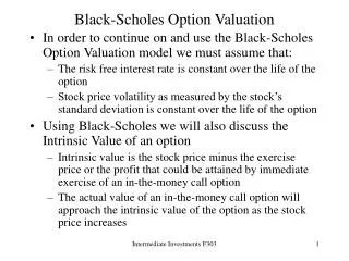
Assumptions: • No dividends are paid on the underlying stock during the life of the option. • Option can only be exercised at expiry (European style). • Efficient markets (Market movements cannot be predicted). • Commissions are non-existent. • Interest rates do not change over the life of the option (and are known) • Stock returns follow a lognormal distribution

Price of the Call ( and r constant) • C=Price of the Call • S=Current Stock Price • T=Time of Expiration • K=Strike Price • r=Risk-free Interest Rate • N()=Cumulative normal distribution function • e=Exponential term (2.7183) • =Volatility

..if r is a function of time

Price of the Put ( and r constant) • P=Price of Put • S=Current Stock Price • T=Time of Expiration • K=Strike Price • r=Risk-free Interest Rate • N=Cumulative normal distribution function • e=Exponential term (2.7183) • =Volatility

Price of Put using Put-Call Parity

Relaxations: • Dividends (Robert Merton) • Taxes and Transaction Costs (Jonathan Ingerson) • Variable Interest Rates (Robert Merton)

Greeks • Greeks are quantities representing the market sensitivity of options or other derivatives. • Delta: sensitivity to changes in price • Gamma: Rate of change in delta • Vega: Sensitivity to volatility • Theta: sensitivity to passage of time • Rho: sensitivity to interest rate

Greeks:

Barrier Options: • A barrier option with payoff Qoand maturity T is a contract which yields a payoff Qo(ST) at maturity T, as long as the spot price St remains in the interval (a(t),b(t)) for all time t[0,T].

Monte-Carlo Methods

Observation: “Because of the difficulty in solving PDEs, numerous methods exist to solve them, including Backlund Transformations, Green’s Function, Integral Transformation, or numerical methods such as finite difference methods.” -www.global-derivatives.com

Orientation: • A technique of employing statistical sampling to approximate solutions to quantitative problems. • Stochastic (nondeterministic) using pseudo-random numbers. • “When number of dimensions (degrees of freedom) in the problem is lerge, PDE’s and numerical integrals become intractable: Monte Carlo methods often give better results” • “MC methods converge to the solutions more quickly than numerical integration methods, require less memory and are easier to program”

Numerical Random Variables • C-library rand() returns an integer value uniformly distributed in [0,RAND_MAX] • To obtain Gaussian random variable: • So that: • Let w1 and w2 be two independent random variables.

Gaussian Random Variable • x is a Gaussian variable with zero mean value, unit variance, and density • Therefore, may be used to simulate

C++ Code:

Initialization: #include <iostream> #include <math.h> #include <stdlib.h> #include <fstream.h> using namespace std; const int M=100; // # of time steps of size dt const int N=50000; // # of stochastic realization const int L=40; // # of sampling point for S const double K = 100; // the strike const double leftS=0, rightS=130; //the barriers const double sigmap=0.2, r=0.1; // volatility, rate const double pi2 =8*atan(1), dt=1./M, sdt =sqrt(dt), eps=1.e-50; const double er=exp(-r);

Function Declarations: double gauss(); double EDOstoch(const double x, int m); //Vanilla double EDOstoch_barrier(const double x, int m, const double Smin, const double Smax); //Barrier double payoff(double s);

Main(): K=100; L=40; 0 – 200, x+=5  40 iterations int main( void ) { ofstream ff("stoch.dat"); for(double x=0.;x<2*K;x+=2*K/L) { // sampling values for x=S double value =0; double y,S ; for(int i=0;i<N;i++) { S=EDOstoch(x,M); //Vanilla Options //S=EDOstoch_barrier(x,M, leftS, rightS); //Barrier double y=0; if (S>= 0) y = er*payoff(S); value += y; } ff << x <<"\t" << value/N << endl; } return 0; } N=50,000; M= 100 er=exp(-r) Payoff=max(S-K, 0) #Ops = 40 X 50,000 = 2,000,000

Gaussian Random Number eps=1.e-50 double gauss() { return sqrt(eps-2.*log(eps+rand()/(double)RAND_MAX)) *cos(rand()*pi2/RAND_MAX); } pi2=8*atan(1)

European Vanilla Call Price () double EDOstoch(const double x, int m) { double S= x; for(int i=0;i<m;i++) S += S*(sigmap*gauss()*sdt+r*dt); return S; // gives S(x, t=m*dt) } m= 100 (dt) Volatility Sqrt(dt) Rate dt= 1.0/M M=500 X: 0 – 200, x+=5  40 iterations

Barrier Call Price() double EDOstoch_barrier(const double x, int m, const double Smin, const double Smax) { if ((x<=Smin)||(x>=Smax)) return -1000; double S= x; for(int i=0;i<m;i++) { if ((S<=Smin)||(S>=Smax)) return -1000; S += S*(sigmap*gauss()*sdt+r*dt); } return S; } double payoff(double s) { if(s>K) return s-K; else return 0;}

Output of the Code: (Vanilla) Figure: Computation of the call price one year to maturity by using the Monte-Carlo algorithm presented in the slides before. The curve displays C versus S. X axis: (20*S)/(K) Y axis: C {payoff K=100,=0.2,r=0.1}

Output of the Code: (Barrier) Figure: Computation of the call price one year to maturity by using the Monte-Carlo algorithm presented in the slides before. The curve displays C versus S. X axis: S a = 0, b = 130 Y axis: C {payoff K=100,=0.2,r=0.1}

Random Variables using GSL #include <gsl/gsl_rng.h> #include <gsl/gsl_rnadist.h> const gsl_rng_type *Tgsl=gsl_rng_default; gsl_rng_env_setup(); gsl_rng *rgsl=gsl_rng_alloc(Tgsl); … double gauss(double dt) { return gsl_ran_gaussian(rgsk, dt); }

Central Limit Theorem • … to come

Variance Reduction • …to come

The Black-Scholes Model for Option Pricing - 2