Download
1 / 20
200 likes | 419 Views
Svetlana Marmutova Laminar flow simulation around circular cylinder 11 of March 2013, Espoo smarmut@uwasa.fi Faculty of Technology. Table of content . Research goals . Table of content . Research goals Model description. Table of content . Research goals Model description

E N D
Svetlana Marmutova Laminar flow simulation around circular cylinder11 of March 2013, Espoo smarmut@uwasa.fi Faculty of Technology
Table of content Research goals
Table of content Research goals Modeldescription
Table of content Research goals Modeldescription Methods
Table of content Research goals Modeldescription Methods Assumptions
Table of content Research goals Modeldescription Methods Assumptions Simulationresults
Table of content Research goals Modeldescription Methods Assumptions Simulationresults Conclusions
Table of content Research goals Modeldescription Methods Assumptions Simulationresults Conclusions Questions for furtherstudies
Research goals • Vertical axis wind turbine power coefficient and efficiency calculation • Steps to achieve the final goal: • Listed cases will be studyed with the use of three computational programs: Comsol, Fluent and Matlab • The first case (static cylinder) is considered in the current presentation. The goal of the presentation is to show and compare the simulation results and uncertainties obtained by means of mentioned programs 2. Cylinder with static axis and freely moving surface Laminar flow 2D; Turbulent flow 2D,3D 3. Windside profile Laminar flow 2D; Turbulent flow 2D,3D 1. Static cylinder Laminar flow 2D; Turbulent flow 2D,3D
2D Laminar flow around static cylinder R=0,05m H=2,2m V=0,4m Uinlet=1m/s Figure 1. Model scheme. • Models and simulation programs: • Comsol, Fluent model: unsteady, laminar, viscous, incompressible, no-slip boundary conditions; • Matlab model: steady, inviscid, incompressible, laminar flow, no-slip boundary conditions, initially calculate stream function;
Methods. Finite difference method (2) (3) Figure 2. Discretization scheme. • Depending on the size of the element (the mesh scale) error accures. Consider element small enough. • Interpolation (in Matlab) • For smoother plot and better result visualization. It should be replaced with the finer grid inside the program code.
Matlab model: • Steady, inviscid, incompressible, laminar flow, no-slip boundary conditions; • Model calculates the stream function; • Stream function on the boundarie (red line) is equal to zero; • Stream function on the boundarie (green line) is calculated through the exact solution. Assumptions (4) (5) Figure 3. Matlab model scheme. (7) (6)
Assumptions (continue) • Figure 4. Matlab model scheme. Differentials can be replaced by difference between grid points according to the finite difference method. • Boundary conditions: for angles 0 , π and on the cylinder surface stream function is equal zero. For R=6 exact solution results are applied. (8)
Assumptions Comsol/Fluent model: • Unsteady, incompressible (ρ=const), laminar with von Karman vortex street creation; • Inlet (velocity is specified), Outlet (gauge pressure is equal to zero), cylinder and tunnel walls (no-slip conditions); • Inertia forces are negleged since the laminar flow is considered; • Incompressibility of the flow is assumed. R=0,05m H=2,2m V=0,4m Uinlet=1m/s Figure 1. Model scheme. (9)
Some Matlab results Figure 5. Matlab velocity profile (m/s). Linear iterpolation index=3
Higher interpolation index • Figure 6. Matlab velocity profile (m/s). Linear iterpolation index=5
Comsol/Fluent Velocity Figure 7. Comsol velocity profile. • Figure 8. Fluent velocity profile (m/s).
Comsol/Fluent Pressure contour Figure 9. Fluent pressure contour (Pa). Figure 10. Comsol pressure contour (Pa).
Conclusions • The model output data was calculated by using Fluent, Matlab and Comsol; • Slightly different results with the use of different programs was observed.
Questions for further studies Interpolation method, which was used to improve data visualization, should be replaced with the finer grid implementation inside the Matlab program code. Previously studied is flow around static cylinder. No-slip boundary conditions were applied.Next case: cylinder under consideration with stationary axis is able to move with the flow around. The boundary conditions on the cylinder surface are unknown: particle’s velocity on the cylinder curface is unknown. Surface characteristics, mechanic moment, cylinder initial velocity should be studyed to find out boundary conditions.