Download
1 / 23
230 likes | 479 Views
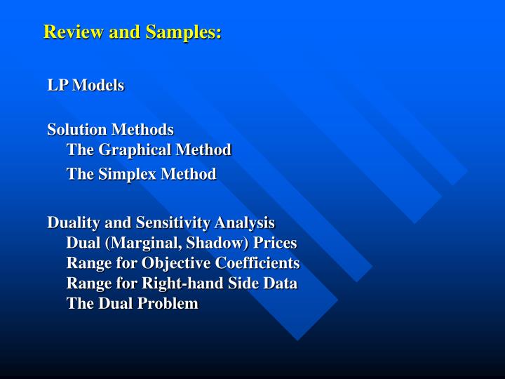
Review and Samples:. LP Models Solution Methods The Graphical Method The Simplex Method Duality and Sensitivity Analysis Dual (Marginal, Shadow) Prices Range for Objective Coefficients Range for Right-hand Side Data The Dual Problem. LP Model: Standard (Inequality) Form. Duality Theory.

E N D
Review and Samples: LP Models Solution MethodsThe Graphical Method The Simplex Method Duality and Sensitivity AnalysisDual (Marginal, Shadow) PricesRange for Objective CoefficientsRange for Right-hand Side DataThe Dual Problem
Duality Theory Standard (Inequality) Primal Form: Dual Form:
Primal-Dual in Matrix Form Standard (Inequality) Primal Form: Dual Form:
Primal-Dual in Matrix Form: Equality Standard (Equality) Primal Form: Dual Form:
Relations Between Primal and Dual 1. The dual of the dual problem is again the primal problem. 2. Either of the two problems has an optimal solution if and only if the other does; if one problem is feasible but unbounded, then the other is infeasible; if one is infeasible, then the other is either infeasible or feasible/unbounded. 3. Weak Duality Theorem: The objective function value of the primal (dual) to be maximized evaluated at any primal (dual) feasible solution cannot exceed the dual (primal) objective function value evaluated at a dual (primal) feasible solution. cTx >= bTy (in the standard equality form)
Relations between Primal and Dual (continued) 4. Strong Duality Theorem: When there is an optimal solution, the optimal objective value of the primal is the same as the optimal objective value of the dual. cTx* = bTy* 5. Complementary Slackness Theorem:Consider an inequality constraint in any LP problem. If that constraint is inactive for an optimal solution to the problem, the corresponding dual variable will be zero in any optimal solution to the dual of that problem. x*j (c-ATy*)j = 0, j=1,…,n.
Optimality Conditions Primal Feasibility: Dual Feasibility: Strong Duality: or Complementary Slackness:
Optimality Conditions Primal Feasibility: Dual Feasibility: Strong Duality: or Complementary Slackness:
Theory of Linear Programming An LP problem falls in one of three cases: • Problem is infeasible: Feasible region is empty. • Problem is unbounded: Feasible region is unbounded towards the optimizing direction. • Problem is feasible and bounded: then there exists an optimal point; an optimal point is on the boundary of the feasible region; and there is always at least one optimal corner point (if the feasible region has a corner point). When the problem is feasible and bounded, • There may be a unique optimal point or multiple optima (alternative optima). • If a corner point is not “worse” than all its neighbor corners, then it is optimal.
Graphical Solution Seeking • Plot the feasible region. • If the region is empty, stop: the problem is infeasible; there must be conflicting constraints in the model. • Plot the objective function contour and choose the optimizing direction. • Determine whether the objective value is bounded or not. If not, stop: the problem is unbounded; there must be mistakes in model formulation. • Determine an optimal corner point. • Identify active constraints at this corner. • Solve simultaneous linear equations for the optimal solution. • Evaluate the objective function at the optimal solution to obtain the optimal value of the problem.
Summary of the Simplex Method for Max (Min) 1.Select a basic feasible solution 2. Express the basic variables in terms of the nonbasic variables, and express the objective function in terms of only nonbasic variables. If all objective coefficients are non-positive (non-negative), then stop: the current basic feasible solution is optimal. Otherwise, select the entering variable such that its coefficient is the greatest (least), and among basic variables select the leaving variable such that it becomes zero first when increasing the entering variable and keeping the other nonbasic variables at zero. If no basic variable becomes zero, then stop: the objective function is unbounded. 3.Goto Step 2.
Complementary Slackness Conditions in the Primal Simplex Method The simplex method maintain the complementary slackness condition, and moving toward
Matrix form of the initial tableau for the inequality standard form Basic Variable x xs RHS Z -c 0 0 xs A I b Matrix form of the tableau with a selected basis B: Basic Variable x xs RHS Z cBB-1A -c cBB-1 cBB-1b xB B-1A B-1 B-1b
The Primal Simplex Method in Tableau 1. Initialization: A:=(A, I) and c:=(c, 0); xB=B-1b 0. 2. Calculate y=cBB-1 and r = yA - c0. If r 0, then optimal and stop; otherwise, goto next step. • Determine the entering basic variable: say select the basic variable with the lowest value in r ; determine the leaving basic variable: whose coefficient in xB reaches zero first as the entering variable increases (use the ratio test of the entering column of B-1A against B-1b).If the increase is unlimited (the column contains all non-positive numbers), then stop, the primal problem is unbounded. Otherwise, using the pivoting procedure to update B, B-1A and B-1b and return to Step 2.
The Dual Simplex Method in Tableau 1. Initialization: A:=(A, I) and c:=(c, 0); y=cBB-1 such that r = yA - c0 2. Calculate xB=B-1b. If xB 0, then optimal and stop; otherwise, goto next step. • Determine the leaving basic variable: say select the basic variable with the lowest value in xB; determine the entering basic variable: whose coefficient in r reaches zero first as the dual variable of the leaving row increases (use the ratio test of the leaving row of B-1A against r).If the increase is unlimited (the row contains all non-negative numbers), then stop, the primal problem is infeasible or dual is unbounded. Otherwise, using the pivoting procedure to update B, B-1A, y=cBB-1 and r = yA – c, and goto Step 2.
Reduced Cost and Objective Coefficient Range • All positive variables have zero reduced cost • In general, the reduced cost of any zero variable is the amount the objective coefficient of that variable would have to change, with all other data held fixed, in order for it to become a positive variable in the OS. If the OS is degenerate, the objective coefficient of a zero variable would have to change by at least, and possibly more that, the reduced cost in order to become a positive variable in the OS. • The objective coefficient ranges give the ranges of the objective function over which no change in the OS will occur. If the OS is degenerate, any objective coefficient must be changed by at least, and possibly more than, the indicated allowable amounts in order to produce a new optimal solution. • One of the “allowable increase and decrease” for a zero variable is infinite and the other is the reduced cost. If a zero variable has zero reduced cost, then there exist an alternative optimal solution.
Dual (Shadow) Price and Constraint RHS Ranges • All inactive constraint have zero dual price • In general, the dual price on a given active constraint is the rate of improvement in the OV as the RHS of the constraint increases with all other data held fixed. If the RHS is decreased, it is the rate at which the OV is impaired. • The constraint RHS ranges give the ranges of the constraint RHS over which no change in the dual price will occur. If the solution is degenerate, the dual price may be valid for one-sided changes in the RHS. • One of the “allowable increase and decrease” for an inactive constraint is infinite and the other equals to the slack or surplus. • In general, when the RHS of an active constraint changes, both the OV and OS will change
Samples: • The Concrete Products Corporation has the capability of producing four types of concrete blocks. Each block must be subjected to three processes: batch mixing, mold vibrating and inspection. The plant manager desires to maximize the profit during the next month. During the upcoming thirty days, he has 800 machine hours available on the batch mixer, 1000 hours on the mold vibrator and 340 man-hours of inspection time. The problem is formulated as follows: max 8x1 + 14x2 + 30x3 + 50x4 S.t. x1 + 2 x2 + 10x3 + 16x4 <= 800 1.5x1 + 2 x2 + 3 x3 + 5 x4 <= 1000 0.5x1 + 0.6x2 + x3 + 2 x4 <= 340 where xi is the production level of the ith product; i = 1, 2, 3, 4.
After solving by the simplex method, the final tableau is Basic x1 x2 x3 x4 x5 x6 x7 Right Z 0 0 28 40 5 2 0 6000 2 0 1 11 19 1.5 -1 0 200 1 1 0 -12 -22 -2 2 0 400 7 0 0 -4 1.6 .1 -.4 1 20
In answering the following question provide a short explanation and computation when needed. 1. By how much must the unit profit on block 3 be increased before it would be profitable to manufacture it ? 2. What must the minimum unit profit on block 2 be so that it remains in the production schedule? 3. If the 800 machine-hours on the batch mixer is uncertain, for what range of machine hours will it remain feasible to produce blocks 1 and 2 ? 4. A competitor located next door has offered the manager additional batch-mixing time at a rate $4.50 per hour. Should he accept his offer? 5. Suppose instead that the competitor offers the manager 250 hours of batch-mixing time for a total $1,100, Should he accept his offer? ( The manager can only accept or reject the extra 250 hours.) 6. The owner has approached the manager with a thought about producing a new type of concrete block that would require 4 hours of batch mixing, 4 hours of molding and 1 hour of inspection per pallet. What should be the profit per pallet if block 5 is to be manufactured? 7. If the next door competitor would like to buy the resources from Concrete Products next month, what would be the fair prices? Formulate it as a linear Program.
The following tableau associated with a LP problem Basic x1 x2 x3 x4 x5 x6 x7 Right Z 0 0 0 g 3 h i 0 2 0 1 0 d 1 0 3 e 3 0 0 1 -2 2 f -1 2 1 1 0 0 0 -1 2 1 3 The entries d, e, f, g, h, i in the tableau are parameters. Each of the following questions is independent, and they all refer to this tableau. Clearly state the range of values of the various parameters that will make the conclusions in the following questions true. 1.The present tableau has a basic feasible solution 2. Row 1 in the present tableau indicates that the problem is infeasible. 3. The current basic solution is feasible, and the present tableau indicates that the problem is unbounded. 4. The current basic solution is feasible, x6 is the entering basic variable, and x3 is the leaving basic variable. 5. The current basic solution is optimal.