Download
1 / 72
730 likes | 906 Views
Heegaard Floer Homology and Existence of Incompressible Tori in Three-manifolds. Eaman Eftekhary IPM, Tehran, Iran. General Construction of HFH.

E N D
Heegaard Floer Homology and Existence of Incompressible Tori in Three-manifolds Eaman Eftekhary IPM, Tehran, Iran
General Construction of HFH • Suppose that Y is a compact oriented three-manifold equipped with a self-indexing Morse function with a unique minimum, a unique maximum, g critical points of index 1 and g critical points of index 2.
General Construction of HFH • Suppose that Y is a compact oriented three-manifold equipped with a self-indexing Morse function h with a unique minimum, a unique maximum, g critical points of index 1 and g critical points of index 2. • The pre-image of 1.5 under h will be a surface of genus g which we denote by S.
h R
Index 3 critical point h R Index 0 critical point
Index 3 critical point Each critical point of Index 1 or 2 will determine a curve on S h R Index 0 critical point
Heegaard diagrams for three-manifolds • Each critical point of index 1 or 2 determines a simple closed curve on the surface S. Denote the curves corresponding to the index 1 critical points by i, i=1,…,g and denote the curves corresponding to the index 2 critical points by i, i=1,…,g.
We add a marked point z to the diagram, placed in the complement of these curves. Think of it as a flow line for the Morse function h, which connects the index 3 critical point to the index 0 critical point.
The marked point z determines a flow line connecting index-0 critical point to the index-3 critical point h z R
We add a marked point z to the diagram, placed in the complement of these curves. Think of it as a flow line for the Morse function h, which connects the index 3 critical point to the index 0 critical point. • The set of data H=(S, (1,2,…,g),(1,2,…,g),z) is called a pointed Heegaard diagram for the three-manifold Y.
A Heegaard Diagram for S1S2 Green curves are curves and the red ones are curves z
Knots in three-dimensional manifolds • Any map embedding S1 in a three-manifold Y determines a homology class H1(Y,Z).
Knots in three-dimensional manifolds • Any map embedding S1 to a three-manifold Y determines a homology class H1(Y,Z). • Any such map which represents the trivial homology class is called a knot.
Trefoil in S3 A projection diagram for the trefoil in the standard sphere
Heegaard diagrams for knots • A pair of marked points on the surface S of a Heegaard diagram H for a three-manifold Y determine a pair of paths between the critical points of indices 0 and 3. These two arcs together determine an image of S1 embedded in Y.
Two points on the surface S determine a knot in Y h z w R
Heegaard diagrams for knots • A Heegaard diagram for a knot K is a set H=(S, (1,2,…,g),(1,2,…,g),z,w) where z,w are two marked points in the complement of the curves 1,2,…,g, and 1,2,…,g on the surface S.
From Heegaard diagrams to Floer homology • Heegaard Floer homology associates a homology theory to any Heegaard diagram with marked points.
From Heegaard diagrams to Floer homology • Heegaard Floer homology associates a homology theory to any Heegaard diagram with marked points. • In order to obtain an invariant of the topological structure, we should show that if two Heegaard diagrams describe the same topological structure (i.e. 3-manifold or knot), the associated homology groups are isomorphic.
Main construction of HFH • Fix a Heegaard diagram H=(S, (1,2,…,g),(1,2,…,g),z1,…,zn)
Main construction of HFH • Fix a Heegaard diagram H=(S, (1,2,…,g),(1,2,…,g),z1,…,zn) • Construct the complex 2g-dimensional smooth manifold X=Symg(S)=(SS…S)/S(g) where S(g) is the permutation group on g letters acting on the g-tuples of points from S.
Main construction of HFH • Fix a Heegaard diagram H=(S, (1,2,…,g),(1,2,…,g),z1,…,zn) • Construct the complex 2g-dimensional smooth manifold X=Symg(S)=(SS…S)/S(g) where S(g) is the permutation group on g letters acting on the g-tuples of points from S. • Every complex structure on S determines a complex structure on X.
Main construction of HFH • Consider the two g-dimensional tori T=12 …g and T=12 …g in Z=SS…S. The projection map from Z to X embeds these two tori in X.
Main construction of HFH • Consider the two g-dimensional tori T=12 …g and T=12 …g in Z=SS…S. The projection map from Z to X embeds these two tori in X. • These tori are totally real sub-manifolds of the complex manifold X.
Main construction of HFH • Consider the two g-dimensional tori T=12 …g and T=12 …g in Z=SS…S. The projection map from Z to X embeds these two tori in X. • These tori are totally real sub-manifolds of the complex manifold X. • If the curves 1,2,…,g meet the curves 1,2,…,g transversally on S, T will meet T transversally in X.
Intersection points of T and T • The complex CF(H), associated with the Heegaard diagram H, is generated by the intersection points x= (x1,x2,…,xg) between T and T . The coefficient ring will be denoted by A, which is a Z[u1,u2,…,un]-module.
Differential of the complex • The differential of this complex should have the following form: The values b(x,y)A should be determined. Then d may be linearly extended to CF(H).
Differential of the complex; b(x,y) • For x,y consider the space x,y of the homotopy types of the disks satisfying the following properties: u:[0,1]RCX u(0,t) , u(1,t) u(s,)=x, u(s,-)=y
Differential of the complex; b(x,y) • For x,y consider the space x,y of the homotopy types of the disks satisfying the following properties: u:[0,1]RCX u(0,t) , u(1,t) u(s,)=x, u(s,-)=y • For each x,y let M() denote the moduli space of holomorphic maps u as above representing the class .
Differential of the complex; b(x,y) • There is an action of R on the moduli space M() by translation of the second component by a constant factor: If u(s,t) is holomorphic, then u(s,t+c) is also holomorphic.
Differential of the complex; b(x,y) • There is an action of R on the moduli space M() by translation of the second component by a constant factor: If u(s,t) is holomorphic, then u(s,t+c) is also holomorphic. • If denotes the formal dimension or expected dimension of M(), then the quotient moduli space is expected to be of dimension -1. We may manage to achieve the correct dimension.
Differential of the complex; b(x,y) • Let n( denote the number of points in the quotient moduli space (counted with a sign) if =1. Otherwise define n(=0.
Differential of the complex; b(x,y) • Let n( denote the number of points in the quotient moduli space (counted with a sign) if =1. Otherwise define n(=0. • Let n(j, denote the intersection number of L(zj)={zj}Symg-1(S) Symg(S)=X with .
Differential of the complex; b(x,y) • Let n( denote the number of points in the quotient moduli space (counted with a sign) if =1. Otherwise define n(=0. • Let n(j, denote the intersection number of L(zj)={zj}Symg-1(S) Symg(S)=X with . • Define b(x,y)=∑ n(.∏j uj n(j, where the sum is over all x,y.
Basic properties • Theorem (Ozsváth-Szabó) The homology groups HF(H,A) of the complex (CF(H),d) are invariants of the pointed Heegaard diagram H. For a three-manifold Y, or a knot (KY), the homology group is in fact independent of the specific Heegaard diagram used for constructing the chain complex and gives homology groups HF(Y,A) and HFK(K,A) respectively.
Refinements of these homology groups • Consider the space Spinc(Y) of Spinc-structures on Y. This is the space of homology classes of nowhere vanishing vector fields on Y. Two non-vanishing vector fields on Y are called homologous if they are isotopic in the complement of a ball in Y.
Refinements of these homology groups • Consider the space Spinc(Y) of Spinc-structures on Y. This is the space of homology classes of nowhere vanishing vector fields on Y. Two non-vanishing vector fields on Y are called homologous if they are isotopic in the complement of a ball in Y. • The marked point z defines a map sz from the set of generators of CF(H) to Spinc(Y): sz:Spinc(Y) defined as follows
Refinements of these homology groups • If x=(x1,x2,…,xg) is an intersection point, then each of xj determines a flow line for the Morse function h connecting one of the index-1 critical points to an index-2 critical point. The marked point z determines a flow line connecting the index-0 critical point to the index-3 critical point. • All together we obtain a union of flow lines joining pairs of critical points of indices of different parity.
Refinements of these homology groups • The gradient vector field may be modified in a neighborhood of these paths to obtain a nowhere vanishing vector field on Y. • The class of this vector field in Spinc(Y) is independent of this modification and is denoted by sz(x). • If x,y are intersection points with x,y, then sz(x) =sz(y).
Refinements of these homology groups • This implies that the homology groups HF(Y,A) decompose according to the Spinc structures over Y: HF(Y,A)=sSpin(Y)HF(Y,A;s) • For each sSpinc(Y) the group HF(Y,A;s) is also an invariant of the three-manifold Y and the Spinc structure s.
Some examples • For S3, Spinc(S3)={s0} and HF(Y,A;s0)=A
Some examples • For S3, Spinc(S3)={s0} and HF(Y,A;s0)=A • For S1S2, Spinc(S1S2)=Z. Let s0 be the Spinc structure such that c1(s0)=0, then for s≠s0, HF(Y,A;s)=0. Furthermore we have HF(Y,A;s0)=AA, where the homological gradings of the two copies of A differ by 1.
Some other simple cases • Lens spaces L(p,q) • S3n(K): the result of n-surgery on alternating knots in S3. The result may be understood in terms of the Alexander polynomial of the knot.
Connected sum formula • Spinc(Y1#Y2)=Spinc(Y1)Spinc(Y2); Maybe the better notation is Spinc(Y1#Y2)=Spinc(Y1)#Spinc(Y2) • HF(Y1#Y2,A;s1#s2)= HF(Y1,A;s1)AHF(Y2,A;s2)
Refinements for knots • Spinc(Y,K) is by definition the space of homology classes of non-vanishing vector fields in the complement of K which converge to the orientation of K.
Refinements for knots • The pair of marked points (z,w) on a Heegaard diagram H for K determine a map from the set of generators x to Spinc(Y,K), denoted by sK(x) Spinc(Y,K).
Refinements for knots • The pair of marked points (z,w) on a Heegaard diagram H for K determine a map from the set of generators x to Spinc(Y,K), denoted by sK(x) Spinc(Y,K). • In the simplest case where A=Z, the coefficient of any y in d(x) is zero, unless sK(x)=sK(y).
Refinements for knots • This is a better refinement in comparison with the previous one for three-manifolds: Spinc(Y,K)=ZSpinc(Y) • In particular for Y=S3 and standard knots we have Spinc(K):=Spinc(S3,K)=Z We restrict ourselves to this case, with A=Z!