Download
1 / 125
1.25k likes | 1.27k Views
This chapter outlines the bisection, Newton’s, and secant methods for locating roots of equations in complex variables. It discusses practical examples, convergence analysis, and the importance of root localization in scientific problem-solving. The chapter also covers the Intermediate-Value Theorem and provides pseudocode for the bisection algorithm. Understanding these methods is crucial for solving nonlinear equations and systems efficiently and accurately.

E N D
CSE 551 Computational Methods 2018/2019 Fall Chapter 4 Locating Roots of Equations
Outline Bisection Method Newton’s Method Secant method
References • W. Cheney, D Kincaid, Numerical Mathematics and Computing, 6ed, • Chapter 3
Bisction Method Introduction Bisection Algor,thm and Pseudocode Examples Convergence Analysis False Position (Regula Falsi) Me4thod and Modifications
Introduction • Let f be a real- or complex-valued function of a real or complex variable • A number r - real or complex - f (r ) = 0 • a root of that equation or a zero of f • e.g., f (x) = 6x2 − 7x + 2 • has 1/2 and 2/3 as zeros, verified • by direct substitution or • by writing f in its factored form: f (x) = (2x − 1)(3x − 2)
g(x) = cos 3x − cos 7x • not only x = 0 • but every integer multiple of π/5 and of π/2 • by the trigonometric identity: • Consequently g(x) = 2 sin(5x) sin(2x)
Why is locating roots important? • solution to a scientific problem is a number • about which - little information • other than that it satisfies some equation • every equation - written • a function stands on one side and zero on the othe • the desired number must be a zero of the function. methods locating zeros of functions • solve such problems
Exercise • Find a scientific or engineering proble m example from your interest area • that is formulated as locating roots of a single nonlinear equation • or a systems of nonlinear equations
In some problems - hand calculator • how to locate zeros of complicated functions?
What is needed • general numerical method • does not depend on special properties of functions • continuity and differentiability - special properties • common attributes of functions that are usually encountered • sort of special property • cannot easily exploit in general-purpose codes • trigonometric identity mentioned previously
Hundreds of methods – available • locating zeros of functions • three of the most useful • the bisection method • Newton’s method • the secant method.
Let f be a function that has values of opposite sign at the two ends of an interval. • Suppose also that f is continuous on that interval • To fix the notation, let a < b and • f (a) f (b) < 0 • It then follows that f has a root in the interval (a, b) • In other words, there must exist a number r that satisfies the two conditions • a < r < b • amd f (r ) = 0.
How is this conclusion reached? • Intermediate-Value Theorem. • If x traverses an interval [a, b], • then the values of f (x) completely fill out the interval between f (a) and f (b) • No intermediate values can be skipped. Hence, a specific function f must take on the value zero somewhere in the interval (a, b) • because f (a) and f (b) are of opposite signs.
Intermediate Value Theorem • A formal statement of the Intermediate-Value Theorem: • If the function f is continuous on the • closed interval [a, b], • and if f (a)y f (b) or f (b) y f (a), • then there exists a point c such that a c b • and f (c) = y.
Bisection Algor,thm and Pseudocode • bisection method exploits this property of continuous functions • At each step algorithm • interval [a, b], values u = f (a) and v = f (b) • u and v satisfy uv < 0 • midpoint of the interval, c = (½) (a + b) • compute w = f (c) • if f (c) = 0 objective fulfilled • usual case: w 0, either wu < 0 or wv < 0 • If wu < 0 - a root of f exists in the interval [a, c]. • store the value of c in b and w in v
If wu > 0 - f has a root in [a, c] • but since wv < 0, f must have a root in [c, b] • store the value of c in a and w in u • either case: the situation at the end of this step is just like that at the beginning except that the final interval is half as large as the initial interval • This step can now be repeated until the interval is satisfactorily small, say |b − a| < (½) × 10−6 • At the end, the best estimate of the root would be (a +b)/2, where [a, b] is the last interval in the procedure.
pseudocode - procedure - general use • a general rule - in programming routines to locate the roots of arbitrary functions: • unnecessary evaluations of the function should be avoided – • costly in terms of computer time • any value of the function - needed later • should be stored rather than recomputed
The procedure to be constructed will • operate on an arbitrary function f . • an interval [a, b] is also specified, • and the number of steps to be taken, nmax, is given. • Pseudocode to perform nmax steps in the bisection algorithm follows:
Pseudocode procedure Bisection( f, a, b, nmax, ε) integer n, nmax; real a, b, c, fa, fb, fc, error fa ← f (a) fb ← f (b) if sign(fa) = sign(fb) then output a, b, fa, fb output “function has same signs at a and b” return end if error ← b − a
for n = 0 to nmax do error ← error/2 c ← a + error fc ← f (c) output n, c, fc, error if |error| < ε then output “convergence” return end if if sign(fa) sign(fc) then b ← c fb ← fc else a ← c fa ← fc end if end for end procedure Bisection
many modifications - enhance the pseudocode: • fa, fb, fc as mnemonics for u, v, w, respectively • Also, we illustrate some techniques of • structured programming and some other alternatives, such as a test for convergence • e.g., if u, v, or w is close to zero - uv or wu may underflow • Similarly, an overflow situation may arise • A test involving the intrinsic function sign could be used to avoid these • difficulties, such as a test that determines whether sign(u) = sign(v) • Here, the iterations • terminate if they exceed nmax or if the error bound (discussed later in this section) is less than ε
Examples • two functions: • for each, seek a zero in a specified interval: f (x) = x3 − 3x +1 on[0, 1] g(x) = x3 − 2 sin x on [0.5, 2]
Solution • write two procedure functions to compute f (x) and g(x) • Then input the initial intervals and the number of steps to be performed in a main program • Since this is a rather simple example, this information could be assigned directly in the main program or by way • of statements in the subprograms rather than being read into the program • Also, depending on the computer language being used, an external or interface statement is needed to tell • the compiler that the parameter f in the bisection procedure is not an ordinary variable • with numerical values but the name of a function procedure defined externally to the main • program. In this example, there would be two of these function procedures and two calls to • the bisection procedure.
A call program or main program that calls the second bisection routine might be written • as follows: program Test Bisection integer n, nmax ← 20 real a, b, ε ← (½)10−6 external function f, g a ← 0.0 b ← 1.0 call Bisection( f, a, b, nmax, ε) a ← 0.5 b ← 2.0 call Bisection(g, a, b, nmax, ε) end program Test Bisection
real function f (x) real x f ← x3 − 3x + 1 end function f real function g(x) real x g ← x3 − 2 sin x end function g
The computer results for the iterative steps of the bisection method for f (x):
To verify these results, • use built-in procedures in mathematical software such as • Matlab, Mathematica, or Maple • to find the desired roots of f and g to be • 0.34729 63553 and 1.23618 3928, respectively • Since f is a polynomial, we can use a routine for finding • numerical approximations to all the zeros of a polynomial function. • However, when more complicated nonpolynomial functions are involved, there is generally no systematic procedure • for finding all zeros. • In this case, a routine can be used to search for zeros (one at • a time), but we have to specify a point at which to start the search, and different starting points may result in the same or different zeros. It may be particularly troublesome to find • all the zeros of a function whose behavior is unknown. • Co
Convergence Analysis • the accuracy bisection method • f - continuous function - takes values of opposite sign at the ends of an interval [a0, b0] • Then there is a root r in [a0, b0] • and if we use the midpoint • c0 = (a0 + b0)/2 as our estimate of r, we have
as illustrated in the figure. If the bisection algorithm is now applied and if the computed • quantities are denoted by a0, b0, c0, a1, b1, c1 and so on, then by the same reasoning, • Since the widths of the intervals are divided by 2 in each step,
Bisection Method Theorem • If the bisection algorithm is applied • to a continuous function f on an interval [a, b], • where f (a) f (b) < 0, • after n steps, an approximate root will have been computed • with error at most (b − a)/2n+1.
If an error tolerance has been prescribed in advance • determine the number of steps required in the bisection method • |r −cn| < ε • solve the following inequality for n: • By taking logarithms (with any convenient base),
Example • How many steps of the bisection algorithm are needed to compute a root of f to full machine • single precision on a 32-bit word-length computer if a = 16 and b = 17?
Solution • The root is between the two binary numbers • a = (10 000.0)2 and b = (10 001.0) 2 • already know five of the binary digits in the answer • Since - can use only 24 bits altogether, • that leaves 19 bits to determine • the last one to be correct, • sthe error • to be less than 2−19 or 2 −20 (being conservative)
Since a 32-bit word-length computer has • a 24-bit mantissa, • expect the answer to have an accuracy of only 2−20. • From the equation above, • (b − a)/2 n+1< ε. • Since b − a = 1 and ε = 2 −20, • 1/2 n+1< 2−20. Taking reciprocals gives 2n+1> 220, or n 20.
Alternatively • Using a basic property of logarithms • log x y= y log x, n >= 20. • each step of the algorithm determines the root with one additional binary digit of precision.
Linear Convergence • A sequence {xn} exhibits linear convergence to a limit x • if there is a constant C in the interval [0, 1) such that • |xn+1 − x| C|xn− x| (n 1) • If this inequality is true for all n, then • |xn+1 − x| C|xn− x| C2|xn-1 − x| · · ·Cn|x1 − x| • Thus, it is a consequence of linear convergence that • |xn+1 − x| ACn (0 C < 1)
he sequence produced by the bisection method obeys Inequality above, as we see from • . However, the sequence need not obey linear convergence.
The bisection method is the simplest way to solve a nonlinear equation f (x) = 0 • It arrives at the root by constraining the interval in which a root lies, and it eventually makes the interval quite small • Because the bisection method halves the width of the interval at each step • one can predict exactly how long it will take to find the root within any desired degree of accuracy • In the bisection method, not every guess is closer to the root than the previous guess because the bisection method does not use the nature of the function itself. • Often the bisection method is used to get close to the root before switching to a faster method.
False Position (Regula Falsi) Method and Modifications • false position method retains the main feature of the bisection method: • a root is trapped in a sequence of intervals of decreasing size • Rather than selecting the midpoint of each interval • this method uses the point where the secant lines intersect the x-axis.
In the figure • the secant line over the interval [a, b] is the chord between (a, f (a)) and (b, f (b)) • The two right triangles in the figure are similar:
compute f (c) and proceed to the next step with the interval [a, c] if f (a) f (c) < 0 • or to the interval [c, b] if f (c) f (b) < 0.
In General • In the general case, the false position method starts with the interval [a0, b0] containing a root: • f (a0) and f (b0) are of opposite signs. • The false position method uses intervals • [ak , bk] that contain roots in almost the same way that the bisection method does. • However, • instead of finding the midpoint of the interval, • it finds where the secant line joining • (ak , f (ak)) and (bk , f (bk)) crosses the x-axis and then selects it to be the new endpoint.
At the kth step, it computes • If f (ak) and f (ck) have the same sign, then • set ak+1 = ckand bk+1 = bk; • otherwise, • set ak+1 = akand bk+1 = ck. • The process is repeated until the root is approximated sufficiently well.
For some functions, the false position method • may repeatedly select the same endpoint • and the process may degrade to linear convergence. • There are various approaches to rectify • this • For example, when the same endpoint is to be retained twice, the modified false position method uses
So rather than selecting points on the same side of the root as the regular false position • method does, the modified false position method changes the slope of the straight line so • that it is closer to the root.
Some variants of the modified false position procedure have superlinear convergence, • which we discuss in Section 3.3. See, for example, Ford [1995]. • Another modified false position method replaces the secant lines by straight lines with ever-smaller slope until the • iterate falls to the opposite side of the root. (See Conte and de Boor [1980].) Early versions • of the false position method date back to a Chinese mathematical text (200 B.C.E. to 100 C.E.) • and an Indian mathematical text (3 B.C.E.).