Download

1 / 104
1.04k likes | 1.2k Views
Microarrays: Common Analysis Approaches. Outline. Missing Value Estimation Differentially Expressed Genes Clustering Algorithms Principal Components Analysis. Missing Data: Outline. Missing data problem, basic concepts and terminology Classes of procedures Case deletion Single imputation

E N D
Outline • Missing Value Estimation • Differentially Expressed Genes • Clustering Algorithms • Principal Components Analysis
Missing Data: Outline • Missing data problem, basic concepts and terminology • Classes of procedures • Case deletion • Single imputation • Filling with zeroes • Row averaging • SVD imputation • KNN imputation • Multiple imputation
The Missing Data Problem Causes for missing data • Low resolution • Image corruption • Dust/scratched slides • Missing measurements Why estimate missing values? • Many algorithms cannot deal with missing values • Distance measure-dependent algorithms(e.g., clustering, similarity searches)
Basic concepts and terminology Statistical overview Missing data mechanism Sample of complete data: θs Sample of incomplete data: θi Population of complete data: θ Sample Need to estimate θ from the incomplete data and investigate its performance over repetitions of the sampling procedure
Basic concepts Y = sample data f(Y;θ) = distribution of sample data θ = parameters to be estimated R = indicators, whether elements of Y are observed or missing g(R|Y) = missing data mechanism (maybe with other params) Y = (Yobs, Ymis) Yobs = observed part of Y Ymis = missing part of Y Goal: Propose methods to estimate θ from Yobs and accurately assess its error
Basic concepts (cont.) Classes of mechanisms (cf. Rubin, 1976, Biometrika) • Missing Completely At Random (MCAR) • g(R|Y) does not depend on Y • Missing At Random (MAR) • g(R|Y) may depend on Yobs but not on Ymis • Missing Not At Random (MNAR) • g(R|Y) depends on Ymis
Example • Suppose we measure age and income of a collection of individuals… • MCAR • The dog ate the response sheets! • MAR • Probability that the income measurement is missing varies according to the age but not income • MNAR • Probability that an income is recorded varies according to the income level with each age group Note: we can disprove MCAR by examining the data, but we cannot disprove MAR or MNAR.
Outline • Missing data problem, basic concepts and terminology • Classes of procedures • Case deletion • Single imputation • Filling with zeroes • Row averaging • SVD imputation • KNN imputation • Multiple imputation
Classes of procedures: Case Deletion • Remove subjects with missing values on any item needed for analysis • Advantages • Easy • Valid analysis under MCAR • OK if proportion of missing cases is small and they are not overly influential • Disadvantages • Can be inefficient, may discard a very high proportion of cases (5669 out of 6178 rows discarded in Spellman yeast data) • May introduce substantial bias, if missing data are not MCAR (complete cases may be un-representative of the population)
Classes of procedures: Single Imputation (I) • Replace with zeroes • Fill-in all missing values with zeroes • Advantages • Easy • Disadvantages • Distorts the data disproportionately (changes statistical properties) • May introduce bias • Why zero?
Classes of procedures: Single Imputation (II) • Row averaging • Replace missing values by the row average for that row • Advantages • Easy • Keeps same mean • Disadvantages • Distorts distributions and relationships between variables x x x x x x x x x x x x x x x x x x x x x x
Classes of procedures: Single Imputation (III) • “Hot deck” imputation • Replace each missing value by a randomly drawn observed value • Advantages • Easy • Preserves distributions very well • Disadvantages • May distort relationships • Can use, e.g., “similar” rows to draw random values from (to help constrain distortion) • Depend on definition of “similar”
Classes of procedures: Single Imputation (IV) • Regression imputation • Fit regression to observed values, use it to obtain predictions for missing ones • SVD imputation • Fill missing entries with regressed values from a set of characteristic patterns, using coefficients determined by the proximity of the missing row to the patterns • KNN imputation (more later) • Isolate rows whose values are similar to those of the one with missing values (choosing (i) similarity measure, and (ii) size of this set) • Fill missing values with averages from this set of genes, with weights inversely proportional to similarities • Computationally intensive • May distort relationships between variables (could use Yimp+random residual)
Classes of procedures: Multiple Imputation • Main Idea • Replace Ymis by M>1 independent draws • {Y1mis,…,YMmis } ~ P(Ymis| Yobs ) • Produce M different versions of complete data • Analyse each one in same fashion and combine results at the end, with standard error estimates (Rubin, 1987) • More difficult to implement • Requires (initially) more computations • More work involved in interpreting results
KNN Imputation • Troyanskaya et al., Bioinformatics, 2001 • The Algorithm • 0. Given gene A with missing values • Find K other genes with values present in experiment 1, with expression most similar to A in other experiments • Weighted average of values in experiment 1 from the K closest genes is used as an estimate for the missing value in A
KNN Imputation: Considerations • K – the number of nearest neighbours • Method appears to be relatively insensitive to K within the range 10-20 • Distance metric to be used for computing gene similarity • Troyanskaya: “Euclidean is sufficient” • No clear comparison or reason – would expect that metric to be used depends on the type of experiment • Not recommended on matrices with less than four columns • Computationally intensive! • ~O(m2n) for m rows and n genes • “3.23 minutes on a Pentium III 500 MHz for 6153 genes, 14 experiments with 10% of the entries missing”
Outline • Missing Value Estimation • Differentially Expressed Genes • Clustering Algorithms • Principal Components Analysis
Identifying Differentially Expressed Genes [Slides courtesy of John Quackenbush, TIGR]
Two vs. Multiple conditions • Two conditions - t-test - Significance analysis of microarrays (SAM) - Volcano Plots • - ANOVA • Multiple conditions - Clustering - K-means - PCA
How Many Replicates?? n = [4(za/2 + zb)2] / [(d/1.4s)2] Where za/2 and zb are normal percentile values at false positive rate aType I error ratefalse negative rate bType II error rate, drepresents the minimum detectable log2 ratio; and s represents the SD of log ratio values. For a = 0.001 and b = 0.05, get za/2 = -3.29 and zb = -1.65. Assume d = 1.0 (2-fold change) and s = 0.25, n = 12 samples (6 query and 6 control) (Simon et al., Genetic Epidemiology 23: 21-36, 2002)
the number of “favorable” outcomes for an event the total number of possible outcomes for that event rf = Probability Distributions • The probability of an event is the likelihood of its occurring. • It is sometimes computed as a relative frequency (rf), where The probability of an event can sometimes be inferred from a “theoretical” probability distribution, such as a normal distribution.
σ = standard deviation of the distribution X = μ (mean of the distribution) Normal Distribution
Mean 1 Mean 2 Population 1 Population 2 Sample mean “s” • Less than a 5 % chance that the sample with mean s came from Population 1 • s is significantly different from Mean 1 at the p < 0.05 significance level. • But we cannot reject the hypothesis that the sample came from Population 2
Probability and Expression Data • Many biological variables, such as height and weight, can reasonably be assumed to approximate the normal distribution. • But expression measurements? Probably not. • Fortunately, many statistical tests are considered to be fairly robust to violations of the normality assumption, and other assumptions used in these tests. • Randomization / resampling based tests can be used to get around the violation of the normality assumption. • Even when parametric statistical tests (the ones that make use of normal and other distributions) are valid, randomization tests are still useful.
s Original data set “fake” s “fake” s “fake” s . . . Randomized “fake” data sets Outline of a Randomisation Test 1. Compute the value of interest (i.e., the test-statistic s) from your data set. 2. Make “fake” data sets from your original data, by taking a random sub-sample of the data, or by re-arranging the data in a random fashion. Re-compute s from the “fake” data set.
Original s value could be significant as it exceeds most of the randomized s values Range of randomized s values Outline of a Randomisation Test (II) 3. Repeat step 2 many times (often several hundred to several thousand times) and record of the “fake” s values from step 2 4. Draw inferences about the significance of your original s value by comparing it with the distribution of the randomized (“fake”) s values
Outline of a Randomisation Test (III) • Rationale • Ideally, we want to know the “behavior” of the larger population from which the sample is drawn, in order to make statistical inferences. • Here, we don’t know that the larger population “behaves” like a normal distribution, or some other idealized distribution. All we have to work with are the data in hand. • Our “fake” data sets are our best guess about this behavior (i.e., if we had been pulling data at random from an infinitely large population, we might expect to get a distribution similar to what we get by pulling random sub-samples, or by reshuffling the order of the data in our sample)
The Problem of Multiple Testing (I) • Let’s imagine there are 10,000 genes on a chip, and • none of them is differentially expressed. • Suppose we use a statistical test for differential expression, where we consider a gene to be differentially expressed if it meets the criterion at a p-value of p < 0.05.
The Problem of Multiple Testing (II) • Let’s say that applying this test to gene “G1” yields a p-value of p = 0.01 • Remember that a p-value of 0.01 means that there is a 1% chance that the gene is not differentially expressed, i.e., • Even though we conclude that the gene is differentially expressed (because p < 0.05), there is a 1% chance that our conclusion is wrong. • We might be willing to live with such a low probability of being wrong • BUT .....
The Problem of Multiple Testing (III) • We are testing 10,000 genes, not just one!!! • Even though none of the genes is differentially expressed, about 5% of the genes (i.e., 500 genes) will be erroneously concluded to be differentially expressed, because we have decided to “live with” a p-value of 0.05 • If only one gene were being studied, a 5% margin of error might not be a big deal, but 500 false conclusions in one study? That doesn’t sound too good.
The Problem of Multiple Testing (IV) • There are “tricks” we can use to reduce the severity of this problem. • They all involve “slashing” the p-value for each test (i.e., gene), so that while the critical p-value for the entire data set might still equal 0.05, each gene will be evaluated at a lower p-value. • We’ll go into some of these techniques later.
The Problem of Multiple Testing (V) • Don’t get too hung up on p-values. • Ultimately, what matters is biological relevance. • P-values should help you evaluate the strength of the evidence, rather than being used as an absolute yardstick of significance. • Statistical significance is not necessarily the same as biological significance.
Finding Significant Genes • Assume we will compare two conditions with multiple replicates for each class • Our goal is to find genes that are significantly different between these classes • These are the genes that we will use for later data mining
Finding Significant Genes (II) ??? • Average Fold Change Difference for each gene • suffers from being arbitrary and not taking into account systematic variation in the data
Finding Significant Genes (III) t = signal = difference between means = <Xq> – <Xc>_ noise variability of groups SE(Xq-Xc) • t-test for each gene • Tests whether the difference between the mean of the query and reference groups are the same • Essentially measures signal-to-noise • Calculate p-value (permutations or distributions) • May suffer from intensity-dependent effects
T-Tests A significant difference Probably not
Group A Group B Exp 1 Exp 2 Exp 3 Exp 4 Exp 5 Exp 6 Exp 1 Exp 2 Exp 5 Exp 3 Exp 4 Exp 6 Gene 1 Gene 1 Gene 2 Gene 2 Gene 3 Gene 3 Gene 4 Gene 4 Gene 5 Gene 5 Gene 6 Gene 6 • Assign experiments to two groups, e.g., in the expression matrix below, assign Experiments 1, 2 and 5 to group A, and experiments 3, 4 and 6 to group B. T-Tests (I) 2. Question: Is mean expression level of a gene in group A significantly different from mean expression level in group B?
T-Tests (II) 3. Calculate t-statistic for each gene 4. Calculate probability value of the t-statistic for each gene either from: A. Theoretical t-distribution OR B. Permutation tests.
Group A Group B Exp 1 Exp 2 Exp 5 Exp 3 Exp 4 Exp 6 Original grouping Gene 1 Group A Group B Exp 1 Exp 2 Exp 5 Exp 3 Exp 4 Exp 6 Randomized grouping Gene 1 T-Tests (III) Permutation tests i) For each gene, compute t-statistic ii) Randomly shuffle the values of the gene between groups A and B, such that the reshuffled groups A and B respectively have the same number of elements as the original groups A and B.
T-Tests (IV) Permutation tests - continued iii) Compute t-statistic for the randomized gene iv) Repeat steps i-iii n times (where n is specified by the user). v) Let x = the number of times the absolute value of the original t-statistic exceeds the absolute values of the randomized t-statistic over n randomizations. vi) Then, the p-value associated with the gene = 1 – (x/n)
T-Tests (V) • 5. Determine whether a gene’s expression levels are significantly different between the two groups by one of three methods: • “Just alpha” (a significance level): If the calculated p-value for a gene is less than or equal to the user-input a (critical p-value), the gene is considered significant. • OR • Use Bonferroni corrections to reduce the probability of erroneously classifying non-significant genes as significant. • B) Standard Bonferroni correction: The user-input alpha is divided by the total number of genes to give a critical p-value that is used as above –> pcritical = a/N.
T-Tests (VI) 5C) Adjusted Bonferroni: i) The t-values for all the genes are ranked in descending order. ii) For the gene with the highest t-value, the critical p-value becomes (a/N), where N is the total number of genes; for the gene with the second-highest t-value, the critical p-value will be (a/[N-1]), and so on.
Finding Significant Genes (IV) • Significance Analysis of Microarrays (SAM)- Uses a modified t-test by estimating and adding a small positive constant to the denominator- Significant genes are those which exceed the expected values from permutation analysis.
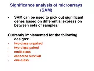
SAM • SAM can be used to select significant genes based on differential expression between sets of conditions • Currently implemented for two-class unpaired design – i.e., we can select genes whose mean expression level is significantly different between two groups of samples (analogous to t-test). • Stanford University, Rob Tibshiranihttp://www-stat.stanford.edu/~tibs/SAM/index.html
SAM • SAM gives estimates of the False Discovery Rate (FDR), which is the proportion of genes likely to have been wrongly identified by chance as being significant. • It is a very interactive algorithm – allows users to dynamically change thresholds for significance (through the tuning parameter delta) after looking at the distribution of the test statistic. • The ability to dynamically alter the input parameters based on immediate visual feedback, even before completing the analysis, should make the data-mining process more sensitive.
Exp 1 Exp 2 Exp 3 Exp 4 Exp 5 Exp 6 Gene 1 Gene 1 Gene 2 Gene 2 Group A Group B Gene 3 Gene 3 Exp 1 Exp 2 Exp 5 Exp 3 Exp 4 Exp 6 Gene 4 Gene 4 Gene 5 Gene 5 Gene 6 Gene 6 • Assign experiments to two groups - in the expression matrix below: Experiments 1, 2 and 5 to group A Experiments 3, 4 and 6 to group B SAM Two-class 2. Question: Is mean expression level of a gene in group A significantly different from mean expression level in group B?
Group A Group B Exp 1 Exp 2 Exp 5 Exp 3 Exp 4 Exp 6 Original grouping Gene 1 Group A Group B Exp 1 Exp 2 Exp 5 Exp 3 Exp 4 Exp 6 Randomized grouping Gene 1 SAM Two-class Permutation tests i) For each gene, compute d-value (analogous to t-statistic). This is the observed d-value for that gene. ii) Randomly shuffle the values of the gene between groups A and B, such that the reshuffled groups A and B have the same number of elements as the original groups A and B. Compute the d-value for each randomized gene