Effective Sales and Operations Planning for Midterm Market Demand Forecasting

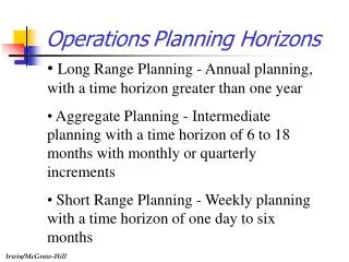
1. SALES AND OPERATIONS PLANNINGAGGREGATE PLANNINGPRODUCTION PLANNINGOPERATIONS PLANNING How to meet effectively and efficiently forecasted market needs(demand) in midterm horizon planning?

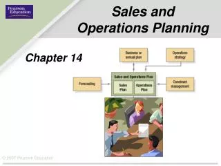
2. Demand Resources Strategic Planning Resource Planning Sales & Operations Plan. (aggregate planning) Forecasts Rough-cut Capacity Plan. Master Production Scheduling (MPS) Customers Orders Detailed Capacity Req. P. Material Requirements Plan. Plan Execution Input /Output Control Purchasing Control Production Control PLANNING AND CONTROL SYSTEM

3. SALES AND OPERATIONS PLANNING • Sales and Operations Planning (SOP). The process of planning future aggregate resources levels so that supply - capacity is in balance with demand • SOP for a manufacturing firm: production plan • SOP for a service firm: staffing plan (workforce plan), • SOP must balance supply with demand to achieve the best compromise between such performance measures as: customer service, work force stability, costs and profit.

4. AGGREGATEPRODUCTION PLANNING Objectives of Aggregate Production Planning: Elaboration of Production Plan which will: • be consistent with strategic plans • meet demand requirements • be realistic within capacity constraints • minimize costs Inputs • Business or annual financial plan • Aggregate demand forecast • Capacity and other resource constraints • Available decision options and their costs Outputs • Production levels for the forthcoming periods • Inventory levels • Workforce levels • Overtimelevels • Subcontracting levels

5. Requirements to production planning • EFFECTIVENESS-meeting of market requirements • FEASIBILITY- production plan should be balanced with availableresources • EFFICIENCY- costsminimizationthroughefficient and rationalresourceutilization

6. According to design similarity According to process similarity According to labour similarity AGGREGATION IN PRODUCTION PLANNING Production planning uses a single measure of output – aggregation of products into common output unit. OBJECTIVE of aggregation – to simplify planning process, more accurate demand forcasts Product family – a group of products that have similar demand requirements and common process, labour and materials requirements. Usually 1-4 families in enterprise Ways of aggregation

7. DEMAND VERS SUPPLY (CAPACITY) STATIC ASPECTS Total Demand in Planning Horizon Case A D = C Case B D  C Case C D  C D C D C D C Time Time Time demand capacity Necessary Condition for Balancing D  C in planning horizon

8. P ZP Czas demand capacity DEMAND VERS CAPACITY (SUPPLY) DYNAMIC ASPECTS Average demand in planning periods Necessary Condition to Balance D  C in planning perid

9. PLANNING DECISION-MAKING OPTIONS Capacity (Production) Options Objective – change capacity model (supply model) Varying workforce size by hiring or layoffs (increase or decrease) Varying production rates through overtime or idle time Using part-time workers Changing inventory levels Subcontractwork to otherfirms Demand Options Objective – change demand model • Vary prices, vary advertising, vary promotion • Back ordering during high- demand periods and carry finished goods inventory – vary the level of customer service • Add contracyclical products - offer complementary products Eight Aggregate Planning Options

10. Contracyclical Demand Products Sales (Units) Total demand 5,000 4,000 Snow scooters 3,000 2,000 1,000 Water scooters) 0 J M M J S N J M M J S N J Time (Months)

11. PRODUCTION PLANNING STRATEGIES LEVEL STRATEGY (level capacity, level scheduling) Maintaining a constant production rate and work force level over the planning horizon Advantages: there are no production increasing and decreasing costs, no hiring and firing costs. Strategy used in many „lean production” enterprises CHASE DEMAND STRATEGY (produce to demand) Strategy that sets production equal to forecasted demand. Involves hiring and laying off employees to match the demand forecast No inventory but there are production increasing and decreasing costs MIXED STRATEGY Strategy that uses two or more options such as production rate, inventory and overtime to set a feasible production plan. Combination of the eight aggregate planning options must be investigated to achieve minimum cost

12. Sales plan Production plan SP PP PP  SP Time Capacity Used Regular Inventory Time Time LEVEL STRATEGY

13. Capacity Used Regular Inventory Time Time CHASE DEMAND STRATEGY Sales plan Production Plan SP PP PP = SP Time

14. Types of costs considered in production planning The planner considers several types of costs when preparing sales and production plans: • Regular- time costs (regular time wages paid to workers) • Overtime costs. Typically 150% of regular- time wages. • Hiring and firing costs. • Inventory holding costs • Backorder and stockout costs.

15. METHODS FOR AGGREGATE PRODUCTION PLANNING GRAPHICAL and CHARTING METHODS MATHEMATICALMETHODS Planning process based on mathematical methods • Linear programming • Transportation method of linear programming • Transportation matrix technique • Dynamic programming • Heuristic techniques (management coefficients model) • Simulation models Planning process based on „trials and errors” approach • Graphical and Charting Methods with Sreadsheeds applications Aggregate planning methods that work with a few variables to compare projected demand with existing capacity. Aggregate planning methods that use production planning models with planning function that produces an optimal plan for minimizing costs.

16. GRAPHICAL AND CHARTING METHODS Charting methods are trial and error approaches that do not guarantee an optimal production plan, but they require only limited computations and can be performer by clerical staff. Steps in the productionplanning • Determine the demandforcast in each period • Determinecapacity for regular time, overtime, and subcontracting in each period. • Findlaborcosts, hiring and layoffcosts and inventory holding costs • Consider policy thatcompanymayapply to the workers and to stocklevels. • Developalternativeplans and examinetheirtotalcosts. Choose the proper plan. DP Cumulative Demand Cumulative Production DC Projected Demand v. Capacity Time Time Graph of Forcast Demand and Capacity Graph of cumulativelevelProduction and Demand

17. PRODUCTION PLANNING FUNCTION MODEL Current status • Productionrates • Workforcesize • Inventory levels Production plan • Productionrates • Workforcesize • Inventorylevels Production planning function Demand forecasts Capacityconstraints • Equipment • Labour • Materials • Overtime • Extra shifts • Subcontracting

18. Planning period (month) 01 02 03 04 05 06 Total Demand forcast [unit] 200 200 300 400 500 200 1.800 D C Time demand capacity Example Capacity Regular labor = 300 unit/m Overtime = 75 unit/m Subcontracting = 50 unit/m Initial inventory = 0 Finalinventory = 0 Costs Regular time production = 20 $/unit Overtime production = 30 $/unit Subcontracting = 40 $/unit Holding = 7 $/unit/m Shortages = 50 $/unit/m Increase production = 35 $/unit/m Decrease production = 35 $/unit/m

19. 200 200 300 400 500 200 1.800 Plan A – LEVEL CAPACITY STRATEGY (pure) PRODUCTION PLAN[units] Planning period DEMAND[units] Regular Inventory Shortages 300 January 100 February 300 200 March 300 200 April 300 100 May 300 0 100 June 300 100 TOTAL [units] 1.800 700 100 Partial costs [$] 36.000 4.900 5.000 TOTAL COSTS = $45.900

20. 200 200 200 200 300 300 400 400 500 500 200 200 1,800 1,800 36,000 Plan B – CHASE DEMAND STRATEGY (pure) PRODUCTION PLAN[units] Planning period Demand[units] Regular Increase Decrease Inventory January 100 February March 100 April 100 May 100 June 300 Total [units] 300 400 Partial costs [$] 10,500 14,000 TOTAL COSTS = $60.500

21. 200 300 200 300 300 300 400 300 500 300 200 300 1,800 1,800 36,000 Plan C – MIXED STRATEGY PRODUCTION PLAN [units] Planning period DEMAND[units] Regulartime Overtime Subcontracting Inventory 100 January February 200 March 200 April 100 May 75 25 0 June 100 TOTAL [unit] 75 25 700 PARTIAL COSTS [unit] 2,250 1,000 4,900 TOTAL COSTS = $44.150

22. Planning period (month) 01 02 03 04 05 06 Total Demand forcast [unit] 200 200 300 400 500 200 1.800 D C Time demand capacity Example of Transportation Matrix use in Production Planning Capacity Regular labor =300 unit/m Overtime =75 unit/m Subcontracting = 50 unit/m Initial inventory = 0 Finalinventory = 0 Costs Regular time production = 2 $/unit Overtime production = 3 $/unit Subcontracting = 6 $/unit Holding = 3 $/unit/m Increase production = 0 $/unit/m Decrease production = 0 $/unit/m Increasing of regular time capacity above 300 units is imposible Zwiększenie zdolności produkcyjnej czasu nominalnego powyżej 300 szt. jest niemożliwe

23. Transportation matrix

24. Transportation matrix 200 100 200 100 0 300 0 50 300 0 0 50 75 0 0 300 50 0 75 0 100 200

25. 200 200 300 400 500 200 1.800 Production Plan PLAN [units] Planning period Demand[units] Inventory Regular Overtime Subcontract January 200 February 200 March 300 50 50 75 75 Appril 300 50 May 300 50 75 June 200 TOTAL [units] 1.500 150 150 125 Partial cost [zł] 3000 450 900 375 Total cost = $ 4725