Download
1 / 50
500 likes | 619 Views
Microgrid Modulation Study. F. High Resolution Sinusoidal Image. High Resolution Image Image FFT. F. Simulated Microgrid Image (Fully Polarized). Fully Polarized Sinusoidal Microgrid Image FFT. Microgrid Demodulation Study. F. Reconstructed sinusoidal s 0 image.

E N D
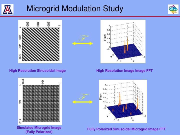
Microgrid Modulation Study F High Resolution Sinusoidal Image High Resolution Image Image FFT F Simulated Microgrid Image(Fully Polarized) Fully Polarized Sinusoidal Microgrid Image FFT
Microgrid Demodulation Study F Reconstructed sinusoidal s0 image. Orientation ~30 deg, freq~.3 cycles/pixel s0 FFT using no interpolation F Reconstructed s1 image. Should be zero. s1 FFT using no interpolation
Systems Model of Microgrid H 45 -45 V Stokes Parameters: Ideal Microgrid Analyzer Vectors: Modulated Analyzer Vector: Analytical Expression for Modulated Intensity: Analyzer Layout on Focal Plane
Analytic Test Scene Test scene using Gaussian stokes parameters. s0 s1 s2 I Intensity output simulated according to:
Data Distribution in Fourier Plane s2-s1 s2+s1 s0 Band limited data easily recovered with use of simple filters
Application to Real Data Microgrid Calibrated Output Fourier Transform of Raw Output In this imagery example, the emissive sphere provides spatially varying angle and degree of polarization. The spatial frequency plane representation of the information clearly shows the base band data (s0) and the horizontal and vertical side lobes (s1and s2).
Edge Artifacts and Polarimetric Aliasing By properly reconstructing the data in the frequency domain (or by using appropriately constructed spatial kernels) polarimetric aliasing can be completely eliminated, leading to ideal reconstruction of band limited imagery Gaussian Kernel NLPN
Modulated Polarimeters • Modulated polarimeters are a second class of device that uses a single detector or detector array to measure an intensity distribution that has been modulated in space, time, and/or wavelength • Spatial Modulation: Prismatic polarimeter, microgrid polarimeter • Temporal Modulation: Rotating retarder, PEM-based devices • Spectral Modulation: Channeled spectropolarimeter • Modulated polarimeters have several inherent strengths: • Inherently spatiotemporally aligned • Can be mechanically rugged and vibration tolerant • Need for cross-calibration of sensors is eliminated • These benefits come at the cost of a reduction in overall system bandwidth
Communications Theory Revisited • Consider two signals present in the same interval of time: • How do we separate the two signals after measurement? • In order to use the available bandwidth of the detector to measure both signals, we have to create multiplexed channels. The simplest and most common method is OFDM, but other methods can also be used.
Frequency Domain Channels • After taking a Fourier transform of the measured intensity, we see that the signals have been separated in frequency S2 S1 Demodulate the s1 channel by homodyning and LPF. • Multiply by cos(2f0t) • Equalize the channels (factor of 2) • Low Pass Filter
Polarimeters as Multiplexed Systems Modulated Analyzer Vector Stokes parameters to be measured Detector response System PSF • System PSF is really a Mueller matrix that alters the polarization state • Consider continuous systems with ideal sampling (h = (x,y,t,), d = (x,y,t,)) • Consider LSI systems, even though this is not always true
Spatial Modulation H 45 -45 V
Spectral Modulation Two high-order, stationary retarders (usually 1:2 or 3:1 thickness ratio) and an analyzer placed in front of a spectrometer. Modulates the spectrum with the Stokes parameters. All Stokes parameters encoded in a single spectrometer measurement. Channels are isolated and Fourier filtered to recover the Stokes vector. Channeled Spectropolarimetry – Slide courtesy Julia Craven-Jones center burst 7 channels 13
Temporal Modulation • The UA-JPL MSPI Polarimeter is an examply of a more complicated modulated system. This 2-channel, temporally modulated polarimeter has analyzer vectors given as:
Consider the DRM: Inverse of the modulator inner product matrix that serves to unmix the Stokes parameter components and equalize their amplitudes Homodyne process that multiplies by the original modulation functions and filters using a rectangular window. For simplicity we consider temporal modulation only, but these concepts are general.
Homodyning • This is nothing more than a homodyne plus a LPF with a rectangular window. We can buy ourselves some flexibility in choosing our LPF by considering the two operations separately
Modulator Inner Product Matrix • The nextstep in the DRM is to compute (WTW)-1 = Z-1. This multiplication also implicitly includes a rectangular-window LPF • In the general case, define the this matrix as: • w is an arbitrary window function that corresponds to the LPF we will use in reconstruction. In the traditional DRM, w is a rectangular window that includes N sample intervals. • For modulation schemes with orthogonal modulators, Z is diagonal, but for more complicated schemes, Z also unmixes the Stokes parameter signals. • `
Generalized Inversion Filtered Equalizer Filtered Homodyne As an aside, this process can be used to create a modified DRM that includes the arbitrary window function with more desirable LPF characteristics.
Example Case – Rotating Retarder • Consider a rotating retarder polarimeter with retardance rotating at angular frequency 2f0.
Band Limited Input Signal • The input signal is fully polarized and band limited:
Measured Signal by Component Each quadrant gives the product an (t) sn (t), and the total signal is obtained by summing these four. The Fourier transform is broken up by parameter.
Reconstructred Signal in Time We see the clear effect of high frequencies that “leak” through and corrupt the reconstruction. We should note that this error is completely avoidable, and is a result of the implied rectangular window used with the DRM method.
Aliasing and Cross Talk in Time When the bandwidth exceeds limits set by the modulation frequency and the sampling frequency, we end up with both aliasing (self-interference) and cross talk that corrupt the reconstructed signal.
Space-Time Modulated Polarimetry • Microgrid Polarimeter modulates in space and creates up to three side bands in spatial frequency space:
Rotating Retarder Polarimeter • The rotating retarder modulates the intensity in time, creating two pairs of complex side bands along the temporal frequency axis
Space-Time Modulation • A rotating retarder followed by a microcrid now creates side bands along the temporal frequency axis for each of the side bands in the spatial frequency plane
Space-Time Modulation Continued • If that retarder is a HWP, we lose the ability to sense s3, but we get the maximum separation of our side bands in the spatio-temporal frequency cube.
Simulation s0 – Microgrid and RR Microgrid RR
Polarization Data (s1) – Microgrid vs RR Microgrid RR
Optimized versus Microgrid (s0) Optimized Microgrid
Optimized versus RR (s0) Optimized RR
Optimized versus Microgrid (s1) Optimized Microgrid
Optimized versus RR (s1) Optimized RR
The Role of the Operator Null Space • Let’s consider different window sizes and shapes in order to assess which method is “better” for any given reconstruction task.
Reconstructed Signal at t= 0 Consider a rectangular window with N . This is just the inner product of the Fourier transforms of A and I. For periodic modulators, we select only the frequencies included in the modulators. All others are in the null space.
Domain of the TraditionalDRM Operator This is just the inner product of the Fourier transforms of A and I. For periodic modulators, we select only the frequencies included in the modulators. All others are in the null space.
Domain of the Band Limited Operator For the band limited inversion operator, the null space includes all frequencies other than the band assigned to a particular Stokes parameter.
Wiener-Helstrum Window • In the general case where we have an expected signal PSD and a known noise PSD, we can construct “optimal” inversion operators that use a window that emphasizes the areas of the spectrum with greatest SNR. An example is the W-H window Assuming uncorrelated, band-limited Stokes parameters with Z independent of time.