Download
1 / 30
300 likes | 327 Views
Explore the input-output relationship in production, long vs. short run dynamics, the law of diminishing returns, marginal product, and maximizing production efficiency. Learn about isoquants, the marginal rate of technical substitution, and its relation to marginal productivity.

E N D
Outline. • The input-output relationship: the production function • Production in the short term • Production in the long term
Production • Production = any activity that creates present or future utility • Production transforms inputs into outputs • Inputs = capital, labour + … • Ignore intermediate goods K, L → (Intermediate goods), K, L → Q proxied by K, L → Q • Firms face technological constraints: feasible production corresponds to the production set
The production function • The production function is the relationship describing the maximum amount of output that can be produced with given quantities of inputs. • It is the boundary of the production set. • The production function can be represented as: Q = f(K,L)
Example: the production of meals. • The production process: Q = 2KL
The long vs. short run • We will distinguish between production in the long run and in the short run • The long run: the shortest period of time necessary to alter the amounts of all inputs. Note that • Variable input = the quantity of which can be altered • Fixed input = the quantity of which cannot be altered during the period • The short run: period during which at least one of the inputs is fixed.
Outline. • Production in the short term • Production in the long term
The production function in the short run • An Example • The production of meals: Q = f(K,L) = 2KL • Assume capital is fixed in the short run at K = K0 = 1. • Then the production function becomes f(K0,L) = 2L
The law of diminishing returns • For L > 4, additional units of labour increase output by a decreasing amount: there are diminishing returns to the variable factor. • Very common property in the short run: see Malthus (1798) • Prediction: At some point, agriculture workers won't produce enough to feed the whole population • Has not happened: why? Growth in the agricultural technology.
Marginal product • Definition: It is the change in the total product that occurs in response to a unit change in the variable input (all other inputs being held fixed) • It is also called marginal productivity. For small changes in the amount of labour: • Slope of the production function.
Average product • Definition: it is the average amount of output produced by each unit of variable input. This is also called average productivity. • Slope of the line joining the origin to the corresponding point on the production function
Example: fishing at both ends of a lake • You are the owner of 4 fishing boats. • 2 of them are fishing at the East end of a very large lake and 2 of them at the West end. • Each boat fishing at the East: 100 pounds of fish per day • Each boat fishing at the West: 120 pounds of fish per day • There is no exhaustion of the fish so that these yields can be maintained forever. Moreover, the fish does not move across the lake. • The question is: should you alter your current allocation of boats? • The intuitive answer is YES because boats at the west end bring more fish than boats at the east end. • However, if the structure of AP and MP are as displayed in Table 2, this answer is wrong.
Table 2 • The current allocation is optimal for the owner of the fish company.
Maximising production • In order to maximise production: • If resources are not perfectly divisible: allocate the next unit of input where its marginal productivity is highest • If resources are perfectly divisible: allocate the resource so that its marginal product is the same in every activity MP(Input)Activity 1 = MP(Input)Activity 2 • Allocating the boats on the basis of their AP is wrong because the MP of a third boat sent to the west is lower than the previous AP. So, it reduces the AP. • Due to diminishing returns to boats given that fish is a fixed amount • If the MP of boats were constant: all boats would be allocated to the West: corner solution ≠ interior solution
Outline. • Production in the long term
Isoquants • In the long run, all inputs can be varied. Q = 2KL • Isoquants • Definition: all combinations of variable inputs that yield a given level of output • They are analogous to the indifference curves for the consumer that would display all combinations of consumption yielding a given level of utility. • We get an isoquant map by moving the isoquants to the northeast as the level of production increases.
The marginal rate of technical substitution • It is the rate at which an input can be exchanged for the other input without altering the production level. • At any given point, it is the absolute value of the slope of the isoquant • It is decreasing along a given isoquant
Graphical definition of the marginal rate of technical substitution
Marginal rate of technical substitution and marginal productivity • There is an important relation between the MRTS and the MP • A variation in output can be decomposed as follows • Along a given isoquant:
Returns to scale • Returns to scale tell us what happens to output when all inputs are increased exactly by the same proportions. • For any a > 1 • Increasing returns to scale: f(aK,aL) > a f(K,L) • Constant returns to scale: f(aK,aL) = a f(K,L) • Decreasing returns to scale: f(aK,aL) < a f(K,L) • Note that in principle, decreasing returnsto scale have nothing to do with the law of diminishing returns.
Some examples of production functions • The Cobb-Douglas production function • where a and b are between 0 and 1 and m > 0 • In this case, returns to scale are given by • if a + b > 1 returns to scale are increasing • if a + b = 1 returns to scale are constant • if a + b < 1 returns to scale are decreasing
Some examples of production functions (ctd) • Isoquants are described by the following expression: • The Leontieff production function Q = min (aK,bL) • Inputs are perfect complements • Isoquants will lie on a locus the equation of which is K = b/a.L • When inputs are perfect substitutes, the production function has the following form Q = aK + aL