Chemical plumes

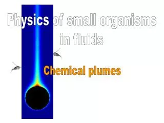
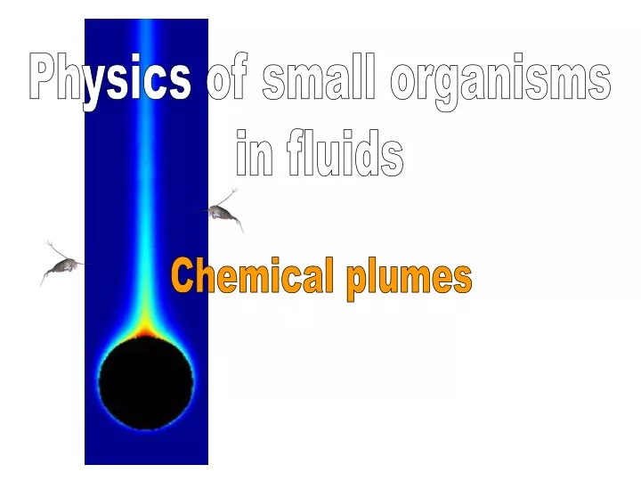
1. Physics of small organisms in fluids Chemical plumes

2. What happens to detritus ? Fecal pellets Marine snow Sinking through water column Remineralization Marine snow aggregates How fast Where To what extent Recycling of nutrients Sequestering of carbon … 5 mm Photo: Alice Alldredge

3. Organisms associated with detritus Rich resource Bacteria Ciliates Dinoflagellates Copepods Larval fish colonizers visitors gulp What mechanisms bring about contact? Plume of released solutes Photo: Alice Alldredge

4. Following a chemical trail First demonstration: The shrimp Segestes acetes following an amino acid trail generated by a sinking wad of cotton that was soaked in a solution of fluorocein and dissolved amino acids. Hamner & Hamner 1977

5. Copepods detect and track chemical plume Temora Kiørboe 2001

6. Physics of small organisms in a fluid: advection - diffusion advection diffusion Pe < 1: diffusion dominates Heuristic says nothing about flux Pe > 1: advection dominates

7. Plume associated with marine snow Re = 1 to 10 Pe≈ 1000

8. Mate tracking

9. Centropages typicus: pheromone trail 17 cm long: 30 sec old Espen Bagoien

10. Sinking rate (w, cm/s) Leakage rate (L, mol/s) The particle: Detection ability – threshold (C* mol/cm3) Swimming speed (v, cm/s) The organism: Turbulence (e cm2/s3, + ….) Diffusion (D, cm2/s) ***** The medium: w Physical parameters for plume encounter What are relevant plume charcteristics ? Approach: analytic and numerical modelling.

11. Particle size dependent properties Sinking rate: Stokes' law Empirical observations Marine snow: a = 0.13, b = 0.26 Fecal pellets: a = 2656, b = 2 Leakage rate: Empirical observations (particle specific leakage rate & size dependent organic matter content) c = 10-12, d = 1.5

12. Detection threshold Species and compound specific Typical free amino acid concentration: 3 10-11 mol cm-3 specific amino acid concentrations < than this Copepod behavioural response (e.g. swarming): 10-11 mol cm-3 Copepod neural response: 10-12 mol cm-3 C* from2 10-12 to 5 10-11 mol cm-3

13. Zero turbulence Length of the plume Time for which plume element remains detectable For marine snow r = 0.5 cm and detection threshold C* = 310-11 mol/cm3 Z0* = 100 cm T0* = 900 sec V0* = 2.5 cm3 (5particle) s0* = 16 cm2 (20 particle) w Jackson & Kiørboe 2004

14. Effect of turbulence on plume Straining and Stretching: Elongates plume lenght 1 Increases concentration gradients – molecular diffusion faster 2 Turbulent shear event Nonuniform: gaps along plume length 3 w + v w Visser & Jackson 2004

15. Direct numerical simulations: solve the Navier Stokes equations Very accurate Hugely expensive Large eddy simulations: solve the Navier Stokes equations for a limited number of scales Relatively accurate Hugely expensive Modelling turbulence Kinematic simulations: analytic expressions that generate turbulence like chaotic stirring Easily done

16. Remember: Kolmogorov spectra theory energy density spectrum, E(k) (L3/T2) Governed by 2 parameters viscosity n dissipation rate e wave number, k (2p/ℓ)

17. Synthetic turbulence simulations + ..... + + k1 k2 kN

18. Synthetic turbulence simulations Wave number, k, ranges from kmin to kmax Assumed energy spectrum: frequency: Amplitude of Fourier coefficients: Random unit vector in 3 D: Random 3 D vectors of magnitude an and bn respectively Fung, 1996. J Geophys Res

19. Path of sinking particle Plume Path of a neutrally plume tracer Particle tracking by Runge-Kutta integration Simulation Particle

20. Plume Plume concentration Gaussian distribution of solute C f r ℓ C* r* l r

21. stretching diffusing Plume construct: stretching and diffusing

22. Mesopelagic (10-8 cm2/s3) Marine snow: r = 0.1 cm w = 0.07 cm/s (60 m/day)

23. Themocline (10-6 cm2/s3) Marine snow: r = 0.1 cm w = 0.07 cm/s (60 m/day)

24. Surface (weak) (10-4 cm2/s3) Marine snow: r = 0.1 cm w = 0.07 cm/s (60 m/day)

25. Surface (strong) (10-2 cm2/s3) Marine snow: r = 0.1 cm w = 0.07 cm/s (60 m/day)

26. Model runs 10 levels of turbulence 3 particle sizes each for marine snow and fecal pellets 4 replicates for each turbulence – size pairing 3 detection threshold Metrics of interest Length; cross-sectional area; degree of fragmentation Natural time scales: turbulence: g = (n / e)1/2 or 1 / mean rate of strain plume: T0* time scale for plume element to drop below threshold of detection. Metric scale: nonturbulent values

27. Total Volume Symbols: different detection threshold Colour: different particle size Rate of turbulent straining Rate of diffusion Fit: p < 0.0001 Visser & Jackson 2004

28. Total Cross section Fit: p < 0.0001 Visser & Jackson 2004

29. 1st Segment Length (distance following plume) Fit: p < 0.0001

30. What can we use this for

31. Copepod encounter with appendicularian houses Appendicularia Copepods Oncaea (cyclopoida) Microsetella (harpacticoida) 0.7 mm Fritillaria borealis Oncaea borealis Microsetella norvegica Oikopleura dioica 5 mm Oncaea similis

32. Remember: Ballistic model variations

33. b s u

34. C* = 3 10-8 µM L = 9 10-14 mol s-1 Maar, Visser, Nielsen, Stips & Saito. accepted

35. v = 0.1 cm s-1 b = 100 µ w = 10 m day-1 Maar, Visser, Nielsen, Stips & Saito. accepted

36. Copepod encounter with appendicularian houses • surface • (above 20 m depth) • =10-2 cm2/s3 g = 1 s-1 0.6 per day per copepod 2.5 per day per appedicularian house 10% per day 10 m day-1 Chouse = 244 m-3 below 30 m 5x Ccopepod = 1000 m-3 • below thermocline • (below 30m depth) • =10-7 cm2/s3 g = 10-3 s-1 4.4 per day per copepod 18 per day per appedicularian house 50% per day

37. Maar, Visser, Nielsen, Stips & Saito. accepted

38. Summary remarks Despite complexity there seem to be global functions relating plume metrics in turbulent and non-turbulent flows. About 50% of the detectable signal becomes disassociated from the particle in high turbulence. Significant advantages can be had for chemosensitive organisms searching for detrital material in low turbulent zones (below the thermocline). Aspects turbulence and its effects on mate finding still to be explored

39. Relative motion Sensing ability Turbulence 1 Encounter rate is everything to plankton Find food Find mates Avoid predators How to

40. 2 Encounter processes Random walks link microscopic (individual) behaviour with macroscopic (population) phenomena Random walk - diffusion Ballistic - Diffusive Scale of interactions

41. Ingestion rate turbulence 3 Encounter rate and turbulence: Dome - shape

42. 4 Patchiness Simple population models + chaotic stirring → complex spatial patterns

43. Thanks