Download
1 / 41
410 likes | 548 Views
Modeling the Plumes of Enceladus. 02/23/2012. Seng K. Yeoh , Todd A. Chapman A dvisors: David B. Goldstein, Philip L. Varghese, Laurence M. Trafton Support is provided by the NASA CDAP and TACC. Enceladus: A Mysterious Moon of Saturn. Credit: NASA/JPL-Caltech.

E N D
Modeling the Plumes of Enceladus 02/23/2012 Seng K. Yeoh, Todd A. Chapman Advisors: David B. Goldstein, Philip L. Varghese, Laurence M. Trafton Support is provided by the NASA CDAP and TACC.
Enceladus: A Mysterious Moon of Saturn Credit: NASA/JPL-Caltech
Some Facts About Enceladus • Diameter ~310 miles • Orbital period of ~1.4 Earth days (~33 hours) • Distance from Saturn center ~4 Saturn radii (~150,000 miles ) • 14th satellite from Saturn • Mean density ~1600 kg/m3 • Gravitational acceleration ~0.113 m/s2 • Bond albedo ~0.99 (value for moon ~ 0.12) Credit: NASA/JPL-Caltech
Diverse Surface Morphology • Northern hemisphere dotted with craters • Almost crater-less south polar region • South polar region also marked by long, parallel fractures known as “tiger stripes” Credit: NASA/JPL-Caltech
Unusual Structure of Saturn’s E Ring • Wide, tenuous, diffuse • Consists mostlyof ice grains • Densest at Enceladus orbit • Narrow E-ring grain distribution (micron-sized) suggests a liquid or vapor source in contrast to broad range by impacts • Enceladus possible major source? Credit: NASA/JPL-Caltech
Quick Facts on Cassini-Huygens 6.7 m • Collaboration between NASA , ESA and ASI • Cassini spacecraft and Huygens probe • Launched October 1997 • Arrived at Saturnian system July 2004 • Extended mission to September 2017 • Three Closest Enceladus Flybys in 2005 • 1st encounter (17 February ) • - Closest approach: 1295 km • - Found tenuous atmosphere • 2nd encounter (9 March) • - Closest approach: 497 km • - Detected southerly water-ion source • 3rd encounter (14 July) • - Closest approach: 168 km • - Discovered active south polar region • - Provided unequivocal evidence of plume over south pole! 4 m Credit: NASA/JPL-Caltech
Some Plume Images The plume you see is actually the dust particle plume as they scatter sun light, not the gas plume! Credit: NASA/JPL-Caltech
CIRS, ISS: Temperature Maps CIRS detected prominent south polar hot spot (>85 K in brightness or blackbody-fit temperature). South polar hot spot Combination of CIRS and ISS found areas with high brightness temperature coincide with tiger stripe fractures. Composite Infrared Spectrometer (CIRS) Imaging Sub-System (ISS) Credit: NASA/JPL-Caltech
UVIS: Stellar Occultation Observations Attenuation of signal of star due to absorption by faint atmosphere during ingress Egress Ultraviolet Imaging Spectrograph (UVIS) Far Ultraviolet Spectrograph (FUV) South pole Ingress Egress Ingress Signal of star disappears because star is behind Enceladus Credit: NASA/JPL-Caltech
INMS, CDA: Plume Composition and Structure • Gas plume composition inferred: ~90% water, ~3% CO2, ~4% CO or N2, ~2% methane and <~1% of acetylene, propane, hydrogen cyanide, and ammonia • Noticeable asymmetry in both water vapor and dust densities • Consistent with a plume source in the south polar region Ion and Neutral Mass Spectrometer (INMS) Cosmic Dust Analyzer (CDA) Credit: NASA/JPL-Caltech
Tiger Stripe fractures may be source of plume! • Strong spatial coincidence with infrared hot spot locations (from CIRS) and locations along tiger stripes • Determined locations and jet orientations of eight strongest sources • Strongest sources being Baghdad and Damascus sulci Yellow Roman numerals: triangulated jet sources (eight sources) Red boxes: hot spots detected by CIRS Credit: NASA/JPL-Caltech Composite Infrared Spectrometer (CIRS)
Overview of Our Plume Model Velocity Distribution Free-molecular model Velocities of Escaping DSMC molecules Point sources Axisymmetric Direct Simulation Monte Carlo (DSMC) model Collisional flow Vent Sub-surface channel
Our Sub-surface Flow Assumptions MaE Vent Conditions: Diameter ~3 m ngas~1021 molecules/m3 Tgas~50 K Vgas ~900 m/s (MaE = 5) Mass flow rate ~0.2 kg/s vent exit Conditions at Vent Exit taken as DSMC input • Circular hole as vent • Water vapor as gas • Channel simply modeled as • converging-diverging nozzle • Short channel (~O(10 m)) • Negligible heat transfer and • frictional effects • Isentropic flow Terrestrial Glacial Crevasse 0.5 m stagnation conditions T0 = 273.16 K p0 = 612 Pa Sub-surface reservoir Enceladus “crevasse” perhaps? Credit: Wikipedia, NASA/JPL-Caltech
Spatial domain is decomposed into cells. • Representative particles move and collide in cells. • Key idea is move and collide steps can be decoupled at timescales much smaller than mean collision time. • Macroscopic quantities (temperature, density, etc.) are obtained by averaging over molecular properties in given cell. • Cells can have a variety of boundary conditions: vacuum, specular/diffuse reflection, or periodic. The Basics of DSMC
DSMC Simulation and Parameters Velocities of Escaping DSMC Particles serve as input to free-molecular model 10 km • Local Knudsen number, Kn = λ/L where λ is mean free path and L is gradient-based length scale, i.e. L = ρ/ . • DSMC domain extends from vent (Kn ~0.001) to 10 km from vent (Kn ~100). • DSMC calculates is multi-staged (8 stages) : - Using a single timestep and a single grid size for entire domain may not be a good idea as properties drop rapidly. - In each stage, timestep is chosen to resolve mean collision time and grid size to resolve mean free path. • Multi-staging works because flow is supersonic (downstream flow does not affect upstream flow). 8th stage: Timestep = 0.005 s Grid size = 20 m 2 m 1st stage: Timestep = 1 x 10⁻⁶ s Grid size = 0.004 m vent Vent Conditions: ngas~1021 molecules/m3 Tgas~50 K Vgas ~900 m/s (MaE = 5)
Free-molecular Model Particle velocities assigned randomly from velocity distribution constructed from escaping DSMC particles • Water particles launched from eight point sources • Locations and jet orientations of sources as determined from Spitale and Porco • Total mass flow rate ~100 kg/s • Each source can have a different mass flow rate (or source rate) • Particles move in ballistic manner under gravitational field • Plasma, radiation, and electromagnetic effects not accounted for (future work)
DSMC Results of Near-field: Number density First 3 stages: vent to 10 m Last 2 stages: 0.5 km to 10 km
DSMC Results of Near-field: Translational Temperature Translational temperature, Ttr is defined as: First 3 stages: vent to 10 m Last 2 stages: 0.5 km to 10 km
DSMC Results of Near-field: Rotational Temperature Rotational temperature, Trot is defined as: First 3 stages: vent to 10 m Last 2 stages: 0.5 km to 10 km
DSMC Results of Near-field: Equilibrium flow • Collisions cause translational and rotational energy modes to exchange energy and equilibrate. • Temperature difference, |Ttr-Trot|, provides a measure of how equilibrium the flow is. First 3 stages: vent to 10 m Last 2 stages: 0.5 km to 10 km
Velocity Components of Escaping DSMC Molecules Normal Velocity (normal to planet surface) North Pole Molecule Velocity Tangential Velocity (tangential to planet surface) Planet surface Planet center
Velocity Distributions for Different Mass Flow Rates 0.001 x ṁnom 0.01 x ṁnom Ultimate speed: = 1005 m/s where γ is the ratio of specific heats (4/3), R is the gas constant (462 J/kg-K) and T0 is the stagnation temperature (273 K) 0.1 x ṁnom nominal (ṁnom ~0.2 kg/s) Flow gets more collisional in near-vent region.
Comparing Simulation Results with In-Situ Data • Modeled two Cassini flybys: i) E3 Flyby: - 12 March 2008 - Closest Approach: 50 km (~31 miles) ii) E5 flyby: - 9 October 2008 - Closest Approach: 21 km (~13 miles) • Water density data was collected to compare to INMS in-situ data • Global sputtering source and E-ring background added to simulation results • Also modeled Gamma Orionis Stellar Occultation on 14 July 2005 • Compare results to UVIS occultation data Ion and Neutral Mass Spectrometer (INMS) Ultraviolet Imaging Spectrograph (UVIS) http://www.youtube.com/watch?v=qZKM8MfUpUs
Gas Column Density Contours Units: molecules/cm2
Simulation Data vs. In-Situ Data Note: All eight sources are of equal strengths. (flyby on 14 July 2005, different from E3 and E5!) before Closest Approach after
Simulation Data vs. In-Situ Data Note: All eight sources are of equal strengths. (closest approach: 50 km) before Closest Approach after
Simulation Data vs. In-Situ Data Note: All eight sources are of equal strengths. (closest approach: 21 km) before Closest Approach after
Examining Time-Variability of Plume • Source strength may vary over time, thus different for each flyby! Our approach to analyzing time-variability of plume: • First, we determine contribution from each source by turn on only a source one by one. • Determine number density by superposition of all source contributions: where Dsimulated(x) is total simulated number density, pn(x) is density contribution from nth source and sn is weight for nth source • Can do superposition of contributions because flow is free-molecular • Smooth and curve-fit INMS data to produce a curve • To find source strengths at each flyby, perform least-squares fitting for Dsimulated(x) to curve • Minimize square of residual: where yi is observations.
Results from Time-Variability Analysis Total strength (kg/s) ~78 ~126
Simulation Data vs. In-Situ Data before Closest Approach after
Simulation Data vs. In-Situ Data before Closest Approach after
Dust Particle Plume Simulations • Particles launched at gas speed (900 m/s) • Low mass loading (<10%) so gas affects dust but not the other way around • Particles are pure ice (density =920 kg/m3) • Particles are moved by gas according to free-molecular drag (diameter-based Knudsen number, KnD ~ O(1000)).
10-nm dust column density Units: molecules/cm2 [km] [km]
50-nm dust column density Units: molecules/cm2 [km] [km]
100-nm dust column density Units: molecules/cm2 [km] [km]
500-nm dust column density Units: molecules/cm2 [km] [km]
1-micron dust column density Units: molecules/cm2 [km] [km]
Conclusions so far • Jet flow out of the vent is very likely to be supersonic. • Enceladus plume varies with time.