Digital Image Fundamentals and Image Enhancement in the Spatial Domain Mohamed N. Ahmed, Ph.D.

1. Digital Image Fundamentals and Image Enhancement in the Spatial Domain Mohamed N. Ahmed, Ph.D. University of Louisville

2. Introduction • An image may be defined as 2D function f(x,y), where x and y are spatial coordinates. • The amplitude of f at any pair (x,y) is called the intensity at that point. When x, y, and f are all finite, discrete quantities, we call the image a digital image. So, a digital image is composed of finite number of elements called picture elements or pixels University of Louisville

3. Introduction • The field of image processing is related to two other fields: image analysis and computer vision Computer Vision Image Processing University of Louisville

4. Introduction • There are three of processes in the continuum • Low Level Processes • Preprocessing, filtering, enhancement • sharpening image Low Level image University of Louisville

5. Introduction • There are three of processes in the continuum • Low Level Processes • Preprocessing, filtering, enhancement • sharpening • Mid Level Processes • segmentation image Low Level image attributes Mid Level image University of Louisville

6. Introduction • There are three of processes in the continuum • Low Level Processes • Preprocessing, filtering, enhancement • sharpening • Mid Level Processes • segmentation • High Level Processes • Recognition image Low Level image attributes Mid Level image recognition High Level attributes University of Louisville

7. Origins of DIP • Newspaper Industry: pictures were sent by Bartlane cable picture between London and New York in early 1920. The introduction of the Bartlane Cable reduced the transmission time from a week to three hours Specialized printing equipment coded pictures for transmission and then reconstructed them at the receiving end. Visual Quality problems 1921 University of Louisville

8. Origins of DIP In 1922, a technique based on photographic reproduction made from tapes perforated at the telegraph receiving terminal was used. This method had better tonal quality and Resolution Had only five gray levels 1922 University of Louisville

9. Origins of DIP Unretouched cable picture of Generals Pershing and Foch transmitted Between London and New York in 1929 Using 15-tone equipment University of Louisville

10. Origins of DIP The first picture of the moon by a US Spacecraft. Ranger 7 took this image On July 31st in 1964. This saw the first use of a digital computer to correct for various types of image distortions inherent in the on-board television camera University of Louisville

11. Applications • X-ray Imaging X-rays are among the oldest sources of EM radiation used for imaging Main usage is in medical imaging (X-rays, CAT scans, angiography) The figure shows some of the applications of X-ray imaging University of Louisville

12. Applications • Inspection Systems Some examples of manufactured goods often checked using digital image processing University of Louisville

13. Applications • Finger Prints • Counterfeiting • License Plate Reading University of Louisville

14. Components of an Image Processing System University of Louisville

15. Steps in Digital Image Processing University of Louisville

16. 2. Digital Image Fundamentals University of Louisville

17. Structure of the Human Eye The eye is nearly a sphere with an Average diameter of 20mm Three membranes enclose the eye: Cornea/Sclera, choroid, and retina. The Cornea is a tough transparent tissue Covering the anterior part of the eye Sclera is an opaque membrane that Covers the rest of the eye The Choroid has the blood supply to the eye University of Louisville

18. Structure of the Human Eye • Continuous with the choroid is the iris which contracts or expands to control the amount of light entering the eye • The lens contains 60 to 70 % water, 6% fat, and protein. • The lens is colored slightly yellow that increases with age • The Lens absorbs 8% of the visible light. The lens also absorbs high amount of infrared and ultra violet of which excessive amounts can damage the eye University of Louisville

19. The Retina • The innermost membrane is the retina • When light is properly focused, the image of an outside object is imaged on the retina • There are discrete light receptors that line the retina: cones and rods University of Louisville

20. Rods and Cones • The cones (7 million) are located in the central portion of the retina (fovea). They are highly sensitive to color • The rods are much larger (75-150 million). They are responsible for giving a general overall picture of the field of view. They are not involved in color vision University of Louisville

21. Image Formation in the Eye University of Louisville

22. Electromagnetic Spectrum University of Louisville

23. Image Acquisition University of Louisville

24. Image Sensors Single Imaging Sensor Line sensor Array of Sensors University of Louisville

25. Image Sensors Single Imaging Sensor Photo Diode Film Sensor University of Louisville

26. Image Sensors Line sensor Image Area Linear Motion University of Louisville

27. Image Sensors Line sensor Image Area Linear Motion University of Louisville

28. Image Sensors Line sensor Image Area Linear Motion University of Louisville

29. Image Sensors Line sensor Image Area Linear Motion University of Louisville

30. Image Sensors Line sensor Image Area Linear Motion University of Louisville

31. Image Sensors Array of Sensors CCD Camera University of Louisville

32. Image Formation Model f(x,y)=i(x,y)r(x,y) where • i(x,y) the amount of illumination incident to the scene 2) r(x,y) the reflectance from the objects University of Louisville

33. Image Formation Model • For Monochrome Images : l = f(x,y) where • l_min < l < l_max • l_min > 0 • l_max should be finite The Interval [l_min, l_max] is called the gray scale In practice, the gray scale is from 0 to L-1, where L is the # of gray levels 0 > Black L-1 > White University of Louisville

34. Image Sampling and Quantization • Sampling is the quantization of coordinates • Quantization is the quantization of gray levels Discrete Continuous Sampling & Quantization University of Louisville

35. Image Sampling and Quantization University of Louisville

36. Sampling and Quantization Continuous Image projected onto a sensor array Results of Sampling and Quantization University of Louisville

37. Effect of Sampling Images up-sampled to 1024x1024 Starting from 1024, 512,256,128,64, and 32 A 1024x1024 image is sub-sampled to 32x32. Number of gray levels is the same University of Louisville

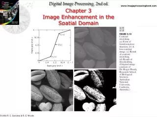
38. Effect of Quantization An X-ray Image represented by different number of gray levels: 256, 128, 64, 32, 16, 8, 4, and 2. University of Louisville

39. Representing Digital Images The result of Sampling and Quantization is a matrix of real Numbers. Here we have an image f(x,y) that was sampled To produce M rows and N columns. University of Louisville

40. Representing Digital Images • There is no requirements about M and N • Usually L= 2k • Dynamic Range : [0, L-1] The number of bits required to store an image b = M x N x kwhere k is the number of bits/pixel Example : The size of a 1024 x 1024 8bits/pixel image is 220 bytes = 1 MBytes University of Louisville

41. Image Storage The number of bits required to store an image b = M x N x kwhere k is the number of bits/pixel The number of storage bits depending on width and height (NxN), and the number Of bits/pixel k. University of Louisville

42. File Formats • PGM/PPM • RAW • JPEG • GIF • TIFF • PDF • EPS University of Louisville

43. File Formats • The TIFF File TIFF -- or Tag Image File Format -- was developed by Aldus Corporation in 1986, specifically for saving images from scanners, frame grabbers, and paint/photo-retouching programs. Today, it is probably the most versatile, reliable, and widely supported bit-mapped format. It is capable of describing bi-level, grayscale, palette-color, and full-color image data in several color spaces. It includes a number of compression schemes and is not tied to specific scanners, printers, or computer display hardware. The TIFF format does have several variations, however, which means that occasionally an application may have trouble opening a TIFF file created by another application or on a different platform University of Louisville

44. File Formats • The GIF FileGIF -- or Graphics Interchange Format -- files define a protocol intended for the on-line transmission and interchange of raster graphic data in a way that is independent of the hardware used in their creation or display. • The GIF format was developed in 1987 by CompuServe for compressing eight-bit images that could be telecommunicated through their service and exchanged among users. • The GIF file is defined in terms of blocks and sub-blocks which contain relevant parameters and data used in the reproduction of a graphic. A GIF data stream is a sequence of protocol blocks and sub-blocks representing a collection of graphics University of Louisville

45. File Formats • The JPEG File JPEG is a standardized image compression mechanism. The name derives from the Joint Photographic Experts Group, the original name of the committee that wrote the standard. In reality, JPEG is not a file format, but rather a method of data encoding used to reduce the size of a data file. It is most commonly used within file formats such as JFIF and TIFF. • JPEG File Interchange Format (JFIF) is a minimal file format which enables JPEG bitstreams to be exchanged between a wide variety of platforms and applications. This minimal format does not include any of the advanced features found in the TIFF JPEG specification or any application specific file format. • JPEG is designed for compressing either full-color or grayscale images of natural, real-world scenes. It works well on photographs, naturalistic artwork, and similar material, but not so well on lettering or simple line art. It is also commonly used for on-line display/transmission; such as on web sites. • A 24-bit image saved in JPEG format can be reduced to about one-twentieth of its original size. University of Louisville

46. Neighbors of a Pixel • A pixel p at coordinates (x,y) has 4 neighbors: (x-1,y), (x+1,y), (x,y-1), (x,y+1). • These pixels are called N4(p) • N8(p) are the eight immediate neighbors of p p University of Louisville

47. Adjacency and Connectivity • Two pixels are connected if: • They are neighbors • Their gray levels satisfy certain conditions (e.g. : g1= g2) *Two pixels p, q are 4 adjacent if *Two pixels p, q are 8 adjacent if University of Louisville

48. Adjacency and Connectivity • Path : • A digital path from p to q is the set of pixel coordinates linking p and q. • Region: • A region is a connected set of pixels p q University of Louisville

49. Distance Measures Assume we have 3 pixels: p:(x,y), q:(s,t) and z:(v,w) A distance function D is a metric that satisfies the following conditions: Example: Euclidean Distance : University of Louisville

50. Distance Measures 2 2 1 2 2 1 0 1 2 2 1 2 2 • City Block Distance : • Chess Board Distance 22 2 2 2 2 1 1 1 2 2 1 0 1 2 2 1 1 1 2 2 2 2 2 2 University of Louisville