Download
1 / 41
410 likes | 541 Views
Characterizing Multi-Decadal Variability in the Southeastern United States. Marcus D. Williams Center for Ocean-Atmospheric Prediction Studies June 2 nd 2010. Outline. Introduction Data Analysis and Results Summary/Conclusions. Introduction and Background.

E N D
Characterizing Multi-Decadal Variability in the Southeastern United States Marcus D. Williams Center for Ocean-Atmospheric Prediction Studies June 2nd 2010
Outline • Introduction • Data • Analysis and Results • Summary/Conclusions
Introduction and Background • To predict future climate variability, and to interpret this variability with appropriate confidence, it is highly desirable to have an understanding of past variability and climate cycles. • The increased global interest in climate change and its impacts has made the need to understand types of long-term variability more pressing. • Regional differences exist in climate variability • Most parts of the world are considered to be warming when examined over a long enough record. • The Southeastern United States along with parts of Europe and Asia have been identified as outliers
Introduction and Background • Easterling et al. 1997 • Analyzed monthly averaged min and max temperatures and DTR at 5400 observing stations around the world • Calculated anomalies from the mean of the base period of 1961 to 1985 for all station in a 5° x 5° lat-lon grid box • P.O.R. of data for study was from 1950-1993
Introduction and Background • In the Southeastern United States (SE US) the El Niño- Southern Oscillation (ENSO) signal is widely recognized as the dominate mode of climate variability. • Ropelewski and Halpert provided research that showed interannual the impacts of ENSO on temperature and precipitation patterns. • Work done by the Intergovernmental Panel on Climate Change addresses climate change on interannual to multidecadal timescales.
Introduction and Background • The analysis presented in this research identifies a mode of variability for the SE US that is of much larger magnitude than the trend, and is influential on a multidecadal timescale. • Analysis has identified a multidecadal regime in the long-term temperature records. • The multidecadal regime shifts from periods warmer than normal temperatures, to periods of colder than normal temperatures.
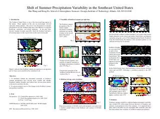
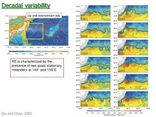
Multidecadal Variability in the Southeast Alabama Annual Temperature Warm period 1920-1957 Cold period 1958-1998
Multidecadal Variability in the Southeast • Same multi-decadal pattern is displayed in the raw, unadjusted station data • 1920-1957: Warm regime (WR) • 1958-1998: Cold regime (CR) Cold regime 1958-1998 Warm regime 1920-1957
Introduction and Background • The mode of climate variability found in my work has been inadequately characterized in the SE US by prior studies • Often times these studies describe variability is in the realm of trend analysis. • The periods over which the trends are fitted can greatly influence the significance or even the sign of the trends. • Work done by Lathers and Palecki, Diaz and Quayle, and other have investigated warm and cool periods Monthly averages for 344 climate divisions was analyzed Many of the studies found the greatest change in summer temperatures • Work done by Lathers and Palecki, Diaz and Quayle, and others have investigated warm and cool periods
Data • Data provided by the National Weather Service Cooperative Observation Program (COOP) • DS 3200 and DS 3206 • DS 3200 is a daily summary of the day data set that consist of 8,000 active observing stations recording daily values of max temp, min temp and precip. • DS 3206 is the data rescue of the data, converting paper records to digital copies
Data Station coverage map of the 104 stations used in the SE US encompassing the states of Alabama, Florida, Georgia, North Carolina, and South Carolina
Data • Stations have data available dating back to at least 1920 and ending in 2007 • Many of the stations used are part of the United States Historical Climate Network (USHCN) • However, for the purpose of this study the daily, unadjusted observations are used • Missing data is addressed by the criteria set forth by Smith (2006)
Data • A multiple linear regression method is used to replace any missing data • Data are pulled from two to five station that lie within a 50-mile radius • Data are de-trended and the seasonal cycle is removed. • Reference stations with correlations of 0.6 or higher are used to calculate the multiple linear regression
Analysis and Results • Goals of my study are to characterize the signal • seasonality, • Is the regime shift seasonal in nature, or is it present in all seasons • spatial extent, • How coherent is the signal of the regime shift • temperature extremes • Is the regime shift affecting the occurrence of extreme temperatures • Analysis and Results • Difference in mean temperatures • Probability distribution function • Ranked sum test • Extreme threshold occurrence • Spatial correlation
Difference in mean temperatures • One of the easiest ways to quantify the differences between the two regimes are to compare the mean temperatures • For each station the mean temperature for the WR is subtracted from the mean temperature for the CR • If the difference is negative the station is assigned a blue dot, positive differences get assigned a red dot • The size of the dot is indicative of the degree difference between the means • Clear that signal is spatially coherent throughout the SE US • Signal strongest in winter minimum and maximum temperatures • Some stations display a difference in means as great as 5°F between the two regimes
Difference of Average Minimum Temperature (1958-1998) period minus (1920-1957) period
Difference of Average Maximum Temperature (1958-1998) period minus (1920-1957) period
Difference in mean temperatures • Two tailed student t-test used to determine if the difference in the means statistically significant t = • Daily min and max temperatures are tested individually for each season • The t scores calculated where on average large and positive • Rarely was a positive t score below 2.5, which suggest significance on the 99% confidence level
Temperature PDF’s • To examine the shift in the regimes over a broad range of temperatures PDF’s are analyzed. • Bin sizes are smallest for summer(3°F) and largest for the fall(8°F). For winter and spring 5°F bins are used. • EX. Camp Hill, AL • Around the 26°F degree temperature bin the chance of occurrence is twice as great for the CR. • WR distribution displays a broad peak, and is skewed towards the warmer range of temperatures • CR distribution has a positive skewness which aligns it with lower temperature values, and also the peak for the CR distribution is much sharper. • Spring and Fall PDF’s show and extension of summer like temperatures • The behavior at the tails of the distribution are highlighted later in the presentation.
Camp Hill, AL Winter Minimum Temperature Distribution 20th percentile shifted from 29°F (WR) to 23°F (CR) 80th percentile shifted from 47°F (WR) to 41°F (CR)
Analysis and Results • All seasons display evidence of a shift between the two regimes for minimum and maximum temperatures • Shift in distributions are largest in winter minimum temperatures. • Spring and Fall distributions display an extension of summer like temperatures • Are the shifts in the distribution statistically significant?
Mann-Whitney-Wilcoxon Ranked Sum Test • Independently discovered in the 1940s by Wilcoxon as well as Mann and Whitney. • Applies to two independent (and non-paired) samples. • The null hypothesis is that the two data samples have been drawn from the same distribution. • U1 = R1−0.5 n1(n1+1), U2 = R2−0.5 n2(n2+1) . • The Ranked Sum Test is to ensure that the shifts in the distribution are statistically significant • To ensure the independence of the data, t is calculated for each station. If a station fails to meet the threshold criteria set, the station is sub-sampled according to tau. • t is the decorrelation time scale
Ranked sum test • Confidence limits are set on a station by station basis for the rejection of the null hypothesis • Each Station is assigned a colored symbol corresponding to a range of confidence limits • Stations with confidence limits 99% are coded red. • Station that lie within the 95-98% confidence interval are yellow • Stations that lie within the 90-94% range are green • Stations <90% are purple
Henderson, NC Fall Maximum Temperature Distribution • Largest shift in Fall maximum temps occur around the higher temperature values • This implies an extension of Summer like temps into the fall season
Threshold occurrence Three occurrences of 95F or greater for the WR compared to no occurrences for the CR