Download
1 / 35
350 likes | 518 Views
Some algorithmic background. Biology 162 Computational Genetics Todd Vision Fall 2004 26 Aug 2004. Some algorithmic background. Algorithms Analysis of time and memory requirements NP completeness Graphs Travelling salesman problem DNA computers Strings and Sequences Recursion.

E N D
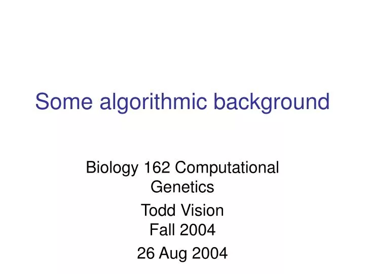
Some algorithmic background Biology 162 Computational Genetics Todd VisionFall 2004 26 Aug 2004
Some algorithmic background • Algorithms • Analysis of time and memory requirements • NP completeness • Graphs • Travelling salesman problem • DNA computers • Strings and Sequences • Recursion
Algorithm • A finite set of rules that gives a sequence of operations for solving a problem suitable for implementation by a computer • A correct algorithm will solve all instances of a problem • An algorithm can be implemented • Multiple ways • In different languages • On different hardware architectures • The choice of algorithm is usually far more important to time/memory usage than implementation
Knuth’s 5 features of an algorithm • Finiteness - guaranteed to terminate • Definiteness - each step precisely defined • Effectiveness - each step must be small • Defined inputs • Defined outputs
Analysis of algorithms • Mathematical description of time and memory requirements • Algorithm efficiency • Time and memory are a function of the size of the problem instancef(x) • Efficiency generally expressed in Big O notation • Assuming the instance is a worst-case scenario • Describes how time/memory scale as problem size grows asymptotically large
Big O notation • O(n), or “order n”, where n is the highest order term in f(x) • For small instances, an O(n2) algorithm may be faster than an O(n) algorithm • The notation does not account for constant factors, which may affect comparisons • The big O notation does not allow one to actually predict the running time or memory usage • Average running time may be much better than worst-case
Algorithm efficiency • An algorithm is efficient if the running time is bounded by a polynomial • O(n4) yes • O(4n) no • O(4log(n)) gray area • Problems are considered to be of class • P if a deterministic efficient algorithm exists • NP if no such algorithm has yet been found • NP-complete if a nondeterministic polynomial time algorithm exists
Are NP-complete problems in class P? • If any NP-complete problem is provably in class P, then all NP-complete problems must be! • Strictly, this applies only to decision problems • Corresponding optimization problems must be at least as hard, and are referred to as NP-hard • Many of the most interesting problems in computational biology are NP-complete or NP-hard
Algorithms without optimality guarantees • Approximation algorithm • For many NP-hard problems, polynomial-time algorithms exist that can provably give answers within some small factor e of the optimal answer • Heuristic algorithm • An algorithm that may be sensible, and may work in practice, but is not necessarily efficient and has no guarantee of finding a solution within e of the optimal one
Travelling salesman problem • A salesman must visit each city on a list exactly once, covering the smallest number of miles in total • Classic NP-hard problem • Excellent approximate algorithms exist • Many computational biology problems are solved by casting them as instances of the TSP and then applying an existing algorithm
Travelling salesman problem 810 New York Chicago 2050 1330 2790 Los Angeles 1090 1400 1610 2720 1540 Dallas Miami 1190
Graph jargon • A graphG(V, E) is composed of a set of vertices (V) and edges(E) • Vertices are also known as nodes • The edges, and thus the graphs, may be • Directed, if edges have a head at one vertex and a tail at the other • Undirected otherwise • The degree of a vertex is the number of adjacent vertices • For directed graphs, vertices have an indegree and an outdegree
Graph jargon • Weighted graphs have a cost or distancew(Ei) on each edge i (as in the TSP) • A path is a list of vertices (v1,v2..vk) where (vi,vi+1) are adjacent • The weight of a path is the sum of the weights on each edge • A cycle is a path which returns to the same vertex • Acyclic graphs have no paths that are cyclic • Acyclic undirected graphs are trees • The phylogenetic trees that biologists know and love • Important data structures
Graph jargon • Connected components are sets of vertices for which • No adjacent vertices are excluded • Do not contain subsets of vertices that are themselves connected components
Eulerian graph • Contains a cycle in which each edge appears exactly once • A Eulerian path can be found with an algorithm that is O(n+m) in the number of vertices n and edges m 3 2 7 8 4 1 6 5
Hamiltonian graph • Contains a cycle in which each vertex appears exactly once • The objective of the TSP is to find a Hamiltonian path with minimal weight • Problems with Hamiltonian paths are NP-hard
DNA computing • In 1994, Leonard Adleman implemented a DNA computer that could solve for a Hamiltonian cycle in a graph
DNA computing • Outline of algorithm • Generate all possible routes • Select itineraries that start with the proper city and end with the final city • Select itineraries with the correct number of cities • Select itineraries that contain each city only once • Each step corresponds to the application of a standard molecular biology reaction
DNA computing Cities are encoded by oligonucleotides Los Angeles GCTACG Chicago CTAGTA Dallas TCGTAC Miami CTACGG New York ATGCCG The path (LA, Chicago, Dallas, Miami, New York) would be: GCTACG CTAGTA TGCTAC CTACGG ATGCCG
DNA computing • Random itineraries obtained by • mixing oligonucleotides encoding both cities and routes in a test tube • Allowing complementary DNA strands to hybridize • Adding ligase to glue the pieces together
DNA computing • Select for paths that start in LA and end in NY • By performing the polymerase chain reaction with LA and NY specific primers X X
DNA computing • Select paths of the appropriate length (5 cities = 30 bases) by isolating the correct band from an electrophoretic gel
DNA computing • Select paths in which each city is represented by affinity purification with probes complementary to each city • A path of length 5 containing each city once must be a Hamiltonian Path
DNA computing • Is this practical? • No. A 200 city HP problem would require more DNA than the weight of the Earth • Is this useful? • Yes. • DNA operations are inherently massively parallel, making simultaneous evaluation of 1015 molecules feasible • Silicon-chip computers perform only sequential operations and cannot deal with large combinatorial problems by exhaustive search
Stretching the analogy • Many biological operations can be thought of in algorithmic terms • Specific proteins act in defined sequences on a variable set of inputs to produce a definite output • Cell division • Neuronal firing • Protein secretion
Segue to sequence analysis • DNA and protein sequences will be the center of our attention for much of the course • We need to be able to precisely describe algorithms that have these molecules as inputs and outputs
Sequences and strings • Biologists and computer scientists use the words string and sequence differently • You will see “sequence” used in both ways in this class • In CS jargon • A stringS is an contiguous ordered set of symbols • A sequence is an ordered set of letters that need not be continuous • If ABCDEFGH is a string • ACEG is a sequence • All strings are sequences, but not all sequences are strings
String jargon • W.r.t. some alphabetA • For DNA, A={a,c,g,t} • For proteins, there are 20 symbols in the alphabet • A DNA string: S=‘acgtgc’ • The length of a string is given by |S|=6 • Index the ith position in S by S[i] • An interval S[i..j] defines a substring of S • S is a superstring of all its component substrings • S[1..j] is a prefix and S[j..|S|] is is a suffix of S
Alignment as a string edit • We can define edit operations on S • Substitution • Insertion • Deletion • Objective functions • One way to formulate the sequence alignment problem is “transform S into S’ with a minimal edit distance” (ie fewest operations) • Equivalently, we can seek an alignment with a maximal score
Pairwise alignment • Scores reflects a ratio of • Probability of alignment under evolutionary model • Probability of a chance alignment • Expressed as a Log Odds, or LOD, ratio • Total score is simply the sum of scores for each edit operation • A brute force algorithm • Enumerate all possible alignments and choose the one(s) with highest score
Dynamic programming • Efficient (ie polynomial-time) algorithm that guarantees finding an optimal pairwise alignment • O(n2) where n is the the length of the sequences • Comes in a few flavors • Global (Needleman-Wunsch) • Local (Smith-Waterman) • Multiple segments • Repeats, overlaps, etc.
Recursion • Principle of dynamic programming is that the solution to a large instance can be recursively found from solutions to smaller instances
Reading assignments • Gibson & Muse, Box 2.1 Pairwise sequence alignment, pgs 72-75. • Durbin R, Eddy S, Krogh A, Mitchison G (1998) “Ch. 2: Pairwise alignment”, pgs, 12-31 in Biological sequence analysis, Cambridge Univ. Press.