Download
1 / 20
200 likes | 315 Views
Fourier Analysis, part II. March 1, 2013. The Lay of the Land. I finally graded the second TOBI production exercise! Let’s check out the all-star team… Also: the first mystery spectrogram has been posted! A Fourier Analysis homework will be handed out after the weekend…

E N D
Fourier Analysis, part II March 1, 2013
The Lay of the Land • I finally graded the second TOBI production exercise! • Let’s check out the all-star team… • Also: the first mystery spectrogram has been posted! • A Fourier Analysis homework will be handed out after the weekend… • For now, you probably have enough to work on. • Today’s goal: further down the rabbit hole of Fourier Analysis. • Any questions so far?
Quick and Dirty Review • The three main elements of Fourier analysis: • A complex wave • Its component waves (the “harmonics”) • Its potential component waves • = the “reference waves” from the last lecture • A complex wave can be created by simply adding together the component waves. • Normally when we do Fourier analysis, though, we want to find out what the component waves are. • The last element is our primary tool: the dot product.
DFT, so far • “Window” the signal • = break it into smaller chunks • Smooth the window reduce the edges to 0. • With the algorithm of your choice! • Determine the components of the smoothed chunk • Calculate the dot product of the chunk with sine and cosine waves of likely component frequencies • Non-components dot product = 0 • Determine the amplitude of each component • = dot product / power of the component • Power = dot product of a wave with itself
Let’s Try Another • Let’s construct another example: 1 Hz sinewave + a 4 Hz cosine wave with half the amplitude. • 1 2 3 4 5 6 7 8 • A 1 Hz 0 .707 1 .707 0 -.707 -1 -.707 • .5*B 4 Hz .5 -.5 .5 -.5 .5 -.5 .5 -.5 • E Sum: .5 .207 1.5 .207 .5 -1.207 -.5 -1.207 • Let’s check the 1 Hz wave first: • E Sum: .5 .207 1.5 .207 .5 -1.207 -.5 -1.207 • A 1 Hz 0 .707 1 .707 0 -.707 -1 -.707 • E*A Dot: 0 .146 1.5 .146 0 .854 .5 .854 • Sum = 4
Yet More Dots • Another example: 1 Hz sinewave + a 4 Hz cosine wave with half the amplitude. • Now let’s check the 4 Hz wave: • E Sum: .5 .207 1.5 .207 .5 -1.207 -.5 -1.207 • B 4 Hz 1 -1 1 -1 1 -1 1 -1 • E*B Dot: .5 -.207 1.5 -.207 .5 1.207 -.5 1.207 • The sum of these products is also 4. • = half of the power of the 4 Hz cosine wave. • The 4 Hz component has half the amplitude of the 4 Hz cosine reference wave. • (we know the reference wave has amplitude 1)
Mopping Up, Part 2 • Our component analysis gave us the following dot products: • E*A = 4 (A = 1 Hz sinewave) • E*B = 4 (B = 4 Hz cosine wave) • Let’s once again normalize these products by dividing them by the power of the “reference” waves: • power (A) = A*A = 4 E*A/A*A = 4/4 = 1 • power (B) = B*B = 8 E*B/B*B = 4/8 = .5 • These ratios are the amplitudes of the component waves. • The 1 Hz sinewave component has amplitude 1 • The 4 Hz cosine wave component has amplitude .5
Footnote • Sinewaves and cosine waves are orthogonal to each other. • The dot product of a sinewave and a cosine wave of the same frequency is 0. • 1 2 3 4 5 6 7 8 • A sin 0 .707 1 .707 0 -.707 -1 -.707 • F cos 1 .707 0 -.707 -1 -.707 0 .707 • A*F Dot: 0 .5 0 -.5 0 .5 0 -.5 • However, adding cosine and sine waves together simply shifts the phase of the complex wave. • Check out different combos in Praat.
Problem #1 • For any given window, we don’t know what the phase shift of each frequency component will be. • Solution: • Calculate the correlation with the sinewave • Calculate the correlation with the cosine wave • Combine the resulting amplitudes with the pythagorean theorem: • Take a look at the java applet online: • http://www.phy.ntnu.edu/tw/ntnujava/index.php?topic=148
Sine + Cosine Example • Let’s add a 1 Hz cosine wave, of amplitude .5, to our previous combination of 1 Hz sine and 4 Hz cosine waves. • 1 2 3 4 5 6 7 8 • C 1+4: 1 -.293 2 -.293 1 -1.707 0 -1.707 • .5*F cos .5 .353 0 -.353 -.5 -.353 0 .353 • G Sum: 1.5 .06 2 -.646 .5 -2.06 0 -1.353 • Let’s check the 1 Hz sine wave again: • G Sum: 1.5 .06 2 -.646 .5 -2.06 0 -1.353 • A 1 Hz 0 .707 1 .707 0 -.707 -1 -.707 • G*A Dot: 0 .043 2 -.457 0 1.457 0 .957 • Sum = 4
Sine + Cosine Example • Now check the 1 Hz cosine wave: • G Sum: 1.5 .06 2 -.646 .5 -2.06 0 -1.353 • F 1 Hz 1 .707 0 -.707 -1 -.707 0 .707 • G*F Dot: 1.5 .043 0 .457 -.5 1.457 0 -.957 • Sum = 2 • Sinewave component amplitude = 4/4 = 1 • Cosine wave component amplitude = 2/4 = .5 • Total amplitude = • Check out the amplitude of the combo in Praat.
In Sum • To perform a Fourier analysis on each (smoothed) chunk of the waveform: • Determine the components of each chunk using the dot product— • Components yield a dot product that is not 0 • Non-components yield a dot product that is 0 • Normalize the amplitude values of the components • Divide the dot products by the power of the reference wave at that frequency • If there are both sine and cosine wave components at a particular frequency: • Combine their amplitudes using the Pythagorean theorem.
Hold On A Second... • What would happen if our window length was 7 samples long, instead of 8? • Back to the 1 Hz and 4 Hz wave combo: • 1 2 3 4 5 6 7 • Sum: 1 -.293 2 -.293 1 -1.707 0 • 2 Hz 0 1 0 -1 0 1 0 • Dot: 0 -.293 0 .293 0 -1.707 0 • The sum of these products is -1.707, not 0. (!?!) • The Fourier approach can only identify component sinewaves that can fit an integer number of cycles into the window.
Frequency Range • Q: What frequencies can we consider in the Fourier analysis? • One possible (but unrealistic) setup: • A window length of .25 seconds • A sampling rate of 20,000 Hz • (Note: 5,000 samples fit into a window) • Longest possible period in window = .25 seconds, so: • Lowest frequency component = 1 / 0.25 = 4 Hz • Nyquist frequency = 10,000 Hz. • A: We can check all frequencies from 4 to 10,000, in steps of 4 Hz. • (10,000 / 4 = 250 possible frequencies)
Frequency Range, Part 2 • Q: What frequencies can we consider in the Fourier analysis? • Another, more realistic possible setup: • A window length of .005 seconds • A sampling rate of 20,000 Hz • (Note: 100 samples fit into a window) • Longest period = .005 seconds, so: • Lowest frequency component = 1 / .005 = 200 Hz! • Nyquist frequency = 10,000 Hz. • A: from 200 to 10,000, in steps of 200 Hz. • (10,000 / 200 = 50 possible frequencies)
Zero Padding • With short window lengths, we miss out on a lot of interesting frequencies… • The solution is to “pad” the window with zeroes, until it’s long enough to enable us to look at an interesting frequency range. • Example: • 1 2 3 4 5 6 7 8 • Sum: 1 -.293 2 -.293 1 -1.707 0 0 • Q: What effect do you think this would have on the power spectrum? • Component frequencies have a reduced amplitude. • Non-component frequencies have a non-zero amplitude.
Industrial Smoothing • Zero-padding “smooths” the spectrum. • Spectral analysis of complex wave formed by 1 Hz and 4 Hz waves, with an 8 Hz sampling rate: 8 sample window 7 sample window, with zero padding
Another Example • Q: What would happen if we padded the window out to 16 samples? • A: More frequencies we can check (resolution = .5 Hz) • Also: even more smoothing • What would happen if we increased the sampling rate? • Upper end of analyzable frequency range increases • ( higher Nyquist frequency) 7 sample window, with zero-padding, 16 Hz sampling rate
Trade-Offs • What happens if we increase the window length? • (independent of zero padding) • A: Increase the maximum analyzable period, so: • Better frequency resolution • ...without the smoothing. • However: • Temporal resolution is worse. • (because the window length is less precise) • Check it out in Praat.
Morals of the Fourier Story • Shorter windows give us: • Better temporal resolution • Worse frequency resolution • = wide-band spectrograms • Longer windows give us: • Better frequency resolution • Worse temporal resolution • = narrow-band spectrograms • Higher sampling rates give us... • A higher limit on frequencies to consider.